7. Financial
You can use the Financial Sticky Note to perform a variety of financial calculations.
Important!
Financial calculation rules and practices can differ according to country, geographic area, or financial institution.
It is up to you to determine whether the calculation results produced by the Financial Sticky Note are compatible with the financial calculation rules that apply to you.
- 7-1. Financial Calculation Basic Operations
- 7-2. Configuring Financial Settings
- 7-3. Simple Interest
- 7-4. Compound Interest
- 7-5. Cash Flow
- 7-6. Amortization
- 7-7. Interest Conversion
- 7-8. Cost/Sell/Margin
- 7-9. Day Count
- 7-10. Depreciation
- 7-11. Bond Calculation
- 7-12. Break-Even Point
- 7-13. Margin of Safety
- 7-14. Operating Leverage
- 7-15. Financial Leverage
- 7-16. Combined Leverage
- 7-17. Quantity Conversion
7-1. Financial Calculation Basic Operations
7-1-1. To select the type of Financial Calculation
1. Click anywhere on the Paper.
• This displays the Sticky Note menu.
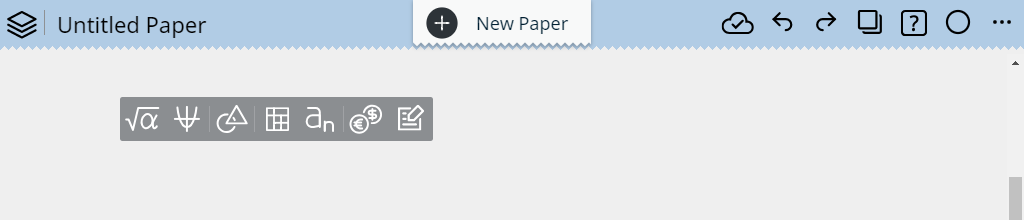
2. Click  .
.
• This creates a Financial Sticky Note and displays a financial calculation type list.
• You can switch between page 1 and page 2 of the type list by clicking [<] and [>].
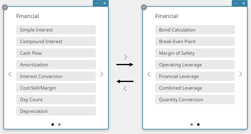
3. Click a financial calculation type.
• This switches to a Financial Sticky Note of the type you clicked. For example, clicking [Simple Interest] switches to a Simple Interest Sticky Note.
7-1-2. Financial Calculation Example
This section uses a Simple Interest Sticky Note to show basic financial calculation operations.
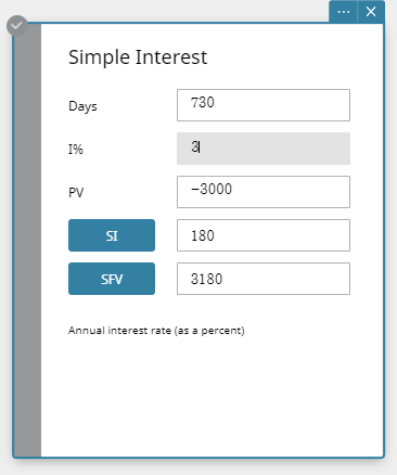
Example:What is the final value after two years (730 days) of a $3,000 investment earning 5% simple interest? Also calculate the final value during the same period for the same investment when the simple interest rate is 3% .
1. Click anywhere on the Paper.
• This displays the Sticky Note menu.
2. Click .
• This creates a Financial Sticky Note and displays a financial calculation type list.
3. Click [Simple Interest].
• This displays the Simple Interest Sticky Note.
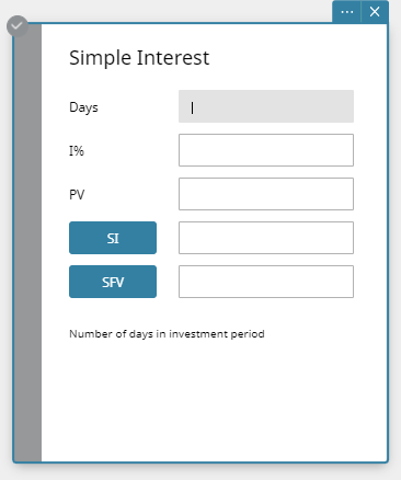
4. Input the following information:
Days $=730$
I%(annual interest rate)$=5$
PV(present value)$=−3000$
5. Click [SI] and then [SFV].
• This displays the calculation results for simple interest (SI) and simple future value (SFV = principal + interest).
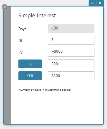
6. Change the I% value to $3$, click [SI], and then [SFV].
• The SI and SFV values are updated in accordance with the new I% value.
7-2. Configuring Financial Settings
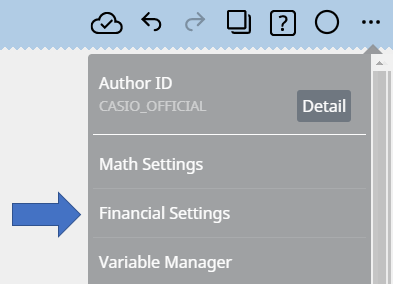
1. Click the Settings button ( ) in the Paper header.

2. Click [Financial Settings].
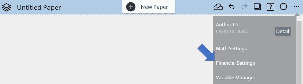
・This displays the Financial Settings dialog box.
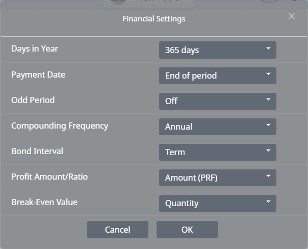
3. You can use this screen to configure settings below.
- Days in Year
360 days: Specifies calculation according to a 360 days. 365 days: Specifies calculation according to a 365 days. - Payment Date
Beginning of period: Specifies the beginning of period as the payment date. End of period: Specifies the end of period as the payment date. - Odd Period
Compound (CI): Specifies compound interest to the odd period when performing a Compound Interest calculation. Simple (SI): Specifies simple interest to the odd period when performing a Compound Interest calculation. Off: Specifies no interest to the odd period when performing a Compound Interest calculation. - Compounding Frequency
Annual: Specifies once a year compounding. Semi-annual: Specifies twice a year compounding. - Bond Interval
Term: Uses a number of payments as term for bond calculation. Date: Uses a date as term for bond calculation. - Profit Amount/Ratio
Amount (PRF): Uses amount (PRF) for break-even point calculations. Ratio (r%): Uses profit ratio (r%) for break-even point calculations. - Break-Even Value
Quantity: Uses quantity for break-even point calculations. Sales: Uses sales amount for break-even point calculations.
4. After settings are the way you want, click [OK].
Note
- Initial default settings are shown below.
Days in Year: 365 days Payment Date: End of period Odd Period: Off Compounding Frequency: Annual Bond Interval: Term Profit Amount/Ratio: Amount (PRF) Break-Even Value: Quantity
- The table below shows setting items for each type of Financial calculation.
Financial Calculation Setting Items Simple Interest Days in Year Compound Interest Payment Date, Odd Period Amortization Payment Date Day Count Days in Year Bond Calculation Days in Year, Compounding Frequency, Bond Interval Break-Even Point Profit Amount/Ratio, Break-Even Value
- There are two ways to change financial settings, described by (a) and (b), below.
- (a) Click
 on the Financial Sticky Note and then change its settings.
Changes made with this method are applied to the Financial Sticky Note being changed only.
- (b) Click in the Paper header, click [Financial Settings], and then change settings.
Changes made with this method are applied to all Financial Sticky Notes that are subsequently created. The changes are not applied to Financial Sticky Notes that were created before the changes were made.
- (a) Click
7-3. Simple Interest
Simple Interest lets you calculate interest (without compounding) based on the number of days money is invested.

7-3-1. Simple Interest Fields
The following fields appear on the Simple Interest calculation.
| Field | Description |
|---|---|
| Days | Number of days in investment period |
| I% | Annual interest rate (as a percent) |
| PV | Present value (initial investment) |
| SI | Calculates and displays simple interest |
| SFV | Calculates and displays simple future value (principal + interest) |
7-3-2. Calculation Formulas
365-day Mode
$ SI' = \cfrac{Dys}{365}\times{PV}\times{i} \qquad (i=\cfrac{I\%}{100}) $
360-day Mode
$ SI' = \cfrac{Dys}{360}\times{PV}\times{i} \qquad (i=\cfrac{I\%}{100}) $
$ SI = -SI' $
$ SFV = -(PV + SI') $
7-4. Compound Interest
Compound Interest lets you calculate interest based on compounding parameters you specify.
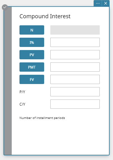
7-4-1. Compound Interest Fields
The following fields appear on the Compound Interest calculation.
| Field | Description |
|---|---|
| N | Number of installment periods |
| I% | Annual interest rate (as a percent) |
| PV | Present value (initial investment) |
| PMT | Amount paid each period |
| FV | Future value |
| P/Y | Number of installment periods per year |
| C/Y | Number of times interest is compounded per year |
7-4-2. Calculation Formulas
・When calculating PV, PMT, FV, n
$ I \% \ne 0 $
$ PV = \cfrac{-\alpha\times{PMT}-\beta\times{FV}}{\gamma} $
$ PMT = \cfrac{-\gamma\times{PV}-\beta\times{FV}}{\alpha} $
$ FV = \cfrac{-\gamma\times{PV}-\alpha\times{PMT}}{\beta} $
$ n = \cfrac{log\left\{\cfrac{(1+iS)\times{PMT}-FV\times{i}}{(1+iS)\times{PMT}+PV\times{i}}\right\}}{\log{(1+i)}} $
$ I \% = 0 $
$ PV = -(PMT\times{n}+FV) $
$ PMT = -\cfrac{PV + FV}{n} $
$ FV = -(PMT\times{n}+PV) $
$ n = -\cfrac{PV+FV}{PMT} $
$ \alpha=(1+i\times{S})\times\cfrac{1-\beta}{i} $
| When “Odd Period” is “Off” | When “Odd Period” is “CI” | When “Odd Period” is “SI” | |
| \( \beta= \) | \( \left(1+i\right)^{-n} \) | \( \left(1+i\right)^{-Ing\left(n\right)} \) | |
| \( \gamma= \) | 1 | \( \left(1+i\right)^{Frac\left(n\right)} \) | \( 1+i \times{Frac\left(n\right)} \) |
| When “Payment Date” is “End of period” | When “Payment Date” is “Beginning of period” | |
| \( S= \) | 0 | 1 |
| When \( P/Y = C/Y = 1 \) | When \( P/Y \neq 1 \) and/or \( C/Y \neq 1 \) | |
| $ i= $ | $ \cfrac{I \%}{100} $ | $ {\left(1+\cfrac{I\%}{100\times\left[C/Y \right]}\right)}^{\cfrac{C/Y}{P/Y}}-1 $ |
・When calculating \( I \) %
i (effective interest rate) is calculated using Newton’s Method.
$ \gamma\times{PV}+\alpha\times{PMT}+\beta\times{FV}=0 $
$ I $ % is calculated from i using the formulas below:
| When \( P/Y = C/Y = 1 \) | When \( P/Y \neq 1 \) and/or \( C/Y \neq 1 \) | |
| $ I \% = $ | $ i\times{10} $ | $ \left( {\left( 1+i \right) }^{\cfrac{P/Y}{C/Y}}-1 \right) \times C/Y \times{100} $ |
Interest (\( I \)%) calculations are performed using Newton’s Method, which produces approximate values whose precision can be affected by various calculation conditions. Interest calculation results produced by this application should be used keeping the above in mind, or results should be confirmed separately.
7-5. Cash Flow
Cash Flow lets you calculate the value of money paid out or received in varying amounts over time.
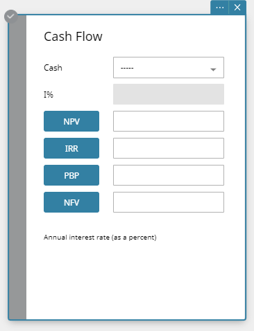
7-5-1. Cash Flow Fields
The following fields appear on the Cash Flow calculation.
| Field | Description |
|---|---|
| Cash | List of income or expenses (up to 80 entries) |
| I% | Annual interest rate (as a percent) |
| NPV | Net present value |
| IRR | Interest rate of return |
| PBP | Payback period |
| NFV | Net future value |
7-5-2. To specify the list to be used by Cash Flow
1. On the Cash Flow Sticky Note, click the "Cash" field.
2. On the menu that appears, click "Add List".
- This displays a Data Sticky Note.
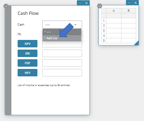
3. Input data to be used by Cash Flow into the Data Sticky Note.
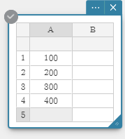
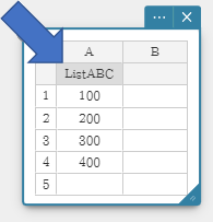
4. Input the list name at the top of data you input.
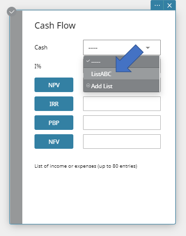
5. On the Cash Flow Sticky Note, click the "Cash" field.
6. On the menu that appears, select the list to be used by Cash Flow.
Note
- For more information about how to edit data values on a Data Sticky Note, see “4-2. Editing Statistical Data Values”.
- When a variable is defined as a list type variable, it will appear in the "Cash" field pulldown menu. You can use a list type variable to perform Cash Flow calculations. For more information about variable types, see “2-11. Using Variable Manager”.
7-5-3. Calculation Formulas
$ NPV=CF_{0}+\cfrac{CF_{1}}{\left(1+i\right)}+\cfrac{CF_{2}}{{\left(1+i\right)}^{2}}+\cfrac{CF_{3}}{{\left(1+i\right)}^{3}}+ \cdots +\cfrac{CF_{n}}{{\left(1+i\right)}^{n}} \qquad \left(i=\cfrac{I\%}{100}\right) $
$ n $: natural number up to 80
$ NFV=NPV\times{\left(1+i\right)}^{n} $
IRR is calculated using Newton’s Method.
$ 0=CF_{0}+\cfrac{CF_{1}}{\left(1+i\right)}+\cfrac{CF_{2}}{{\left(1+i\right)}^{2}}+\cfrac{CF_{3}}{{\left(1+i\right)}^{3}}+ \cdots +\cfrac{CF_{n}}{{\left(1+i\right)}^{n}} $
In this formula, NPV = 0, and the value of IRR is equivalent to i×100. It should be noted, however, that minute fractional values tend to accumulate during the subsequent calculations performed automatically, so NPV never actually reaches exactly zero. IRR becomes more accurate the closer that NPV approaches to zero.
$ PBP=\begin{cases}0 .................. \left(CF_{0}\geq0\right)\\n-\cfrac{NPV_{n}}{NPV_{n+1}-NPV_{n}}...\left(Other\space than\space those\space above\right)\end{cases} $
$ n $: smallest positive integer that satisfies the conditions
$ NPV_{n}\leq 0 $, $0 \leq NPV_{n+1} $, or 0
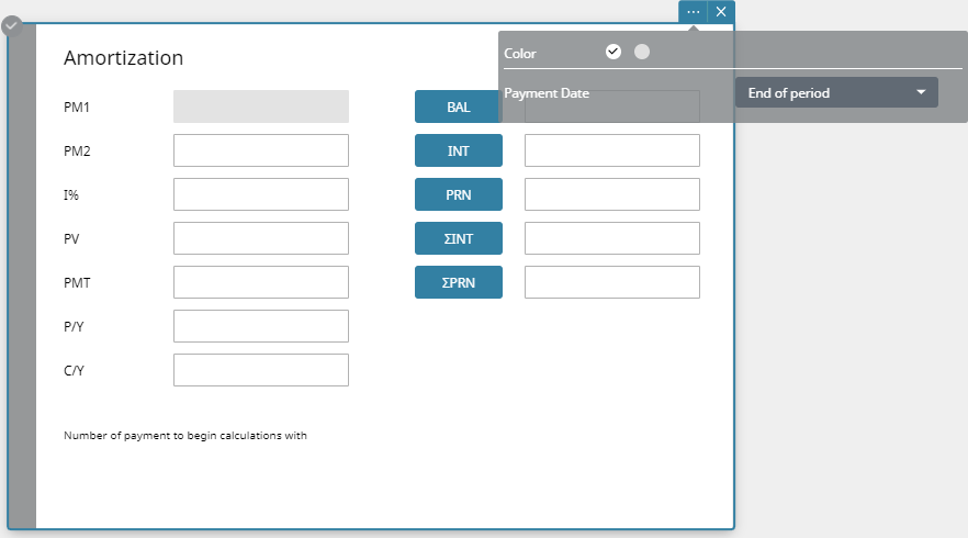
7-6. Amortization
Amortization can be used to calculate the interest and principal paid for a particular year, the total interest and total interest paid for a certain period (year), and the outstanding principal.
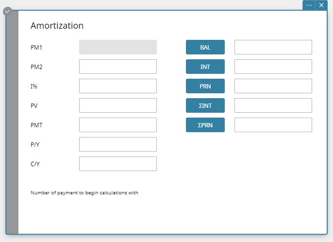
7-6-1. Amortization Fields
The following fields appear on the Amortization calculation.
| Field | Description |
|---|---|
| PM1 | Number of first installment period in interval under consideration |
| PM2 | Number of last installment period in interval under consideration |
| I% | Annual interest rate (as a percent) |
| PV | Present value (initial investment) |
| PMT | Amount paid each period |
| P/Y | Number of installment periods per year |
| C/Y | Number of times interest is compounded per year |
| BAL | Balance of principal after PM2 |
| INT | Interest portion of PM1 |
| PRN | Principal portion of PM1 |
| ΣINT | Total interest paid from PM1 to PM2 (inclusive) |
| ΣPRM | Total principal paid from PM1 to PM2 (inclusive) |
7-6-2. Calculation Formulas
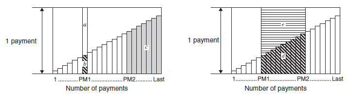
| a: |
Interest portion of payment PM1 (INT) \( INT_{PM1}=\mid{BAL_{PM1-1} \times i}\mid\times\left(PMT_{sign}\right) \) |
| b: |
Principal portion of payment PM1 (PRN) \( PRN_{PM1}=PMT+BAL_{PM1-1}\times{i} \) |
| c: |
Principal balance upon completion of payment PM2 (BAL) \( BAL_{PM2}=BAL_{PM2-1}+PRN_{PM2} \) |
| d: |
Total principal paid from payment PM1 to payment PM2 (ΣPRN) \( \sum_{PM1}^{PM2}PRN=PRN_{PM1}+PRN_{PM1+1}+ \) ... \( +PRN_{PM2} \) |
| e: |
Total interest paid from payment PM1 to payment PM2 (ΣINT) ・a + b = one repayment (PMT) \( \sum_{PM1}^{PM2}INT=INT_{PM1}+INT_{PM1+1}+...+INT_{PM2} \) \( BAL_{0}=PV................ \) Payment Date: End of period (See "7-2. Configuring Financial Settings".) \( INT_{1}=0,PRN_{1}=PMT... \) Payment Date: Beginning of period (See "7-2. Configuring Financial Settings".) |
Converting between the Nominal Interest Rate and Effective Interest Rate
The nominal interest rate (\( I \)% value input by user) is converted to an effective interest rate (\( I \)%') for installment loans where the number of annual payments (P/Y) is different from the number of annual compoundings calculation periods (C/Y).
After conversion from the nominal interest rate to the effective interest rate, i is calculated using the formula below. Next, the calculated i is applied to the Amortization formula. For information about formulas, see "7-6-2. Calculation Formulas".
7-7. Interest Conversion
Interest Conversion lets you calculate the effective or nominal interest rate for interest that is compounded multiple times during a year.
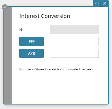
7-7-1. Interest Conversion Fields
The following fields appear on the Interest Conversion calculation.
| Field | Description |
|---|---|
| N | Number of times interest is compounded per year |
| EFF | Effective interest rate (as a percent) |
| APR | Nominal interest rate (as a percent) |
7-7-2. Calculation Formulas
$ APR=\left[{\left(1+\cfrac{EFF}{100}\right)}^{\cfrac{1}{n}}-1\right]\times{n}\times100 $
7-8. Cost/Sell/Margin
Cost/Sell/Margin lets you calculate the cost, selling price, or margin of profit on an item, given the other two values.
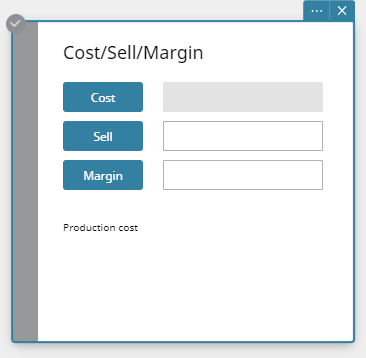
7-8-1. Cost/Sell/Margin Fields
The following fields appear on the Cost/Sell/Margin calculation.
| Field | Description |
|---|---|
| Cost | Production cost |
| Sell | Selling price |
| Margin | Margin of profit (portion of selling price not absorbed by cost of production) |
7-8-2. Calculation Formulas
$ SEL=\cfrac{CST}{1-\cfrac{MRG}{100}} $
$ MRG\left(\%\right)=\left(1-\cfrac{CST}{SEL}\right)\times100 $
7-9. Day Count
Day Count lets you calculate the number of days between two dates, or the date that is a specified number of days from another date.
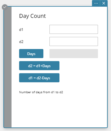
7-9-1. Day Count Fields
The following fields appear on the Day Count calculation.
| Field | Description |
|---|---|
| d1 | Date 1 |
| d2 | Date 2 |
| Days | Number of days from d1 to d2 |
7-10. Depreciation
Depreciation lets you calculate the amount that a business expense can be offset by income (depreciated) over a given year.
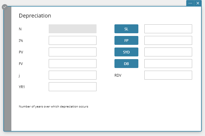
Note
- You can also click [SL] to calculate depreciation using straight-line method, [FP] using fixed-percentage method, or [DB] using declining-balance method. Each depreciation method will produce a different residual value after depreciation (RDV) for the applicable year (j).
7-10-1. Depreciation Fields
The following fields appear on the Depreciation calculation.
| Field | Description |
|---|---|
| N | Number of years over which depreciation occurs |
| I% | Depreciation rate (Fixed-Percentage Method or Declining-Balance Method) |
| PV | Present value (initial investment) |
| FV | Future value (residual value) |
| \( j \) | Year for which depreciation is being calculated |
| YR1 | Number of depreciable months in first year |
| SL | Calculate depreciation for year j using the straight-line method |
| FP | Calculate depreciation for year j using the fixed-percentage method |
| SYD | Calculate depreciation for year j using the sum-of-the-years’-digits method |
| DB | Calculate depreciation for year j calculated using the declining-balance method |
| RDV | Residual value after depreciation for year \( j \) |
7-10-2. Calculation Formulas
・Straight-Line Method
$ SL_{j}=\cfrac{\left(PV-FV\right)}{n} $
$ SL_{n+1}=\cfrac{\left(PV-FV\right)}{n}\times\cfrac{12-YR1}{12} $
$ (YR1 \ne 12) $
・Fixed-Percentage Method
$ FP_{j}=\left(RDV_{j-1}+FV\right)\times\cfrac{I\%}{100} $
$ FP_{n+1}=RDV_{n} \qquad \left(YR1\neq12\right) $
$ RDV_{1}=PV-FV-FP_{1} $
$ RDV_{j}=RDV_{j-1}-FP_{j} $
$ RDV_{n+1}=0 \qquad \left(YR1\neq12\right) $
・Sum-of-the-Years’-Digits Method
$ n'=n-\cfrac{YR1}{12} $
$ Z'=\cfrac{\left(Intg\left(n'\right)+1\right)\left(Intg\left(n'\right)+2\times{Frac\left(n'\right)}\right)}{2} $
$ SYD_{1}=\cfrac{n}{Z}\times\cfrac{YR1}{12}\left(PV-FV\right) $
$ SYD_{j}=\left(\cfrac{n'-j+2}{Z'}\right)\left(PV-FV-SYD_{1}\right) \qquad \left(j\neq1\right) $
$ SYD_{n+1}=\left(\cfrac{n'-\left(n+1\right)+2}{Z'}\right)\left(PV-FV-SYD_{1}\right)\times\cfrac{12-YR1}{12} \qquad \left(YR1\neq12\right) $
$ RDV_{1} = PV-FV-SYD_{1} $
$ RDV_{j} = RDV_{j-1}-SYD_{j} $
・Declining-Balance Method
$ RDV_{1}=PV-FV-DB_{1} $
$ DB_{j}=\left(RDV_{j-1}+FV\right)\times\cfrac{I\%}{100n} $
$ RDV_{j}=RDV_{j-1}-DB_{j} $
$ DB_{n+1}=RDV_{n} \qquad \left(YR1\neq12\right) $
$ RDV_{n+1}=0 \qquad \left(YR1\neq12\right) $
7-11. Bond Calculation
Bond Calculation lets you calculate the purchase price or the annual yield of a bond.
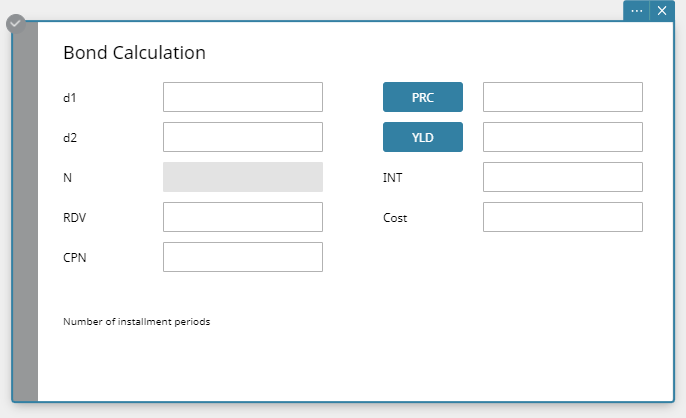
7-11-1. Bond Calculation Fields
The following fields appear on the Bond Calculation.
| Field | Description |
|---|---|
| d1 | Purchase date |
| d2 | Redemption date |
| N | Number of periods |
| RDV | Redemption value |
| CPN | Annual coupon rate |
| PRC | Price of bond |
| YLD | Annual yield (as a percent) |
| INT | Interest accumulated during partial year portion of investment period |
| Cost | Cost of bond (price plus partial year interest) |
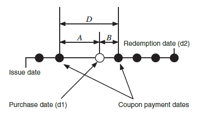
7-11-2. Calculation Formulas
・Terms in the formulas
- $PRC$ : price per $100 of face value
- $RDV$ : redemption price per $100 of face value
- $CPN$ : coupon rate (%)
- $YLD$ : annual yield (%)
- $M$ : number of coupon payments per year
(1 = Annual, 2 = Semi-annual) - $N$ : number of coupon payments until maturity (n is used when “Term” is specified for “Bond Interval”.)
- $INT$ : accrued interest
- $CST$ : price including interest
- $A$ : accrued days
- $D$ : number of days in coupon period where settlement occurs
- $B$ : number of days from purchase date until next coupon payment date $=D–A$
・$PRC$ when “Date” is specified for “Bond Interval”
For one or fewer coupon period to redemption:
$ PRC=\cfrac{RDV+CPN/M}{1+\left(B/D\times\left(YLD/100\right)/M\right)}+A/D\times{CPN/M} $
For more than one coupon period to redemption:
$ PRC=-\cfrac{RDV}{{\left(1+\left(YLD/100\right)/M\right)}^{ \left( N-1+B/D \right) }} \quad - \sum_{k=1}^N\cfrac{CPN/M}{{\left(1+\left(YLD/100\right)/M\right)}^{\left( N-1+B/D \right) }} \quad + A/D\times{CPN/M} $
$ INT=-A/D\times{CPN/M} \qquad CST=PRC\times{INT} $
・$PRC$ when “Term” is specified for “Bond Interval”
$ PRC=-\cfrac{RDV}{{\left(1+\left(YLD/100\right)/M\right)}^{n}} \quad -\sum_{k=1}^N\cfrac{CPN/M}{{\left(1+\left(YLD/100\right)/M\right)}^{k}} \qquad INT=0 \qquad CST=PRC $
・$YLD$
The Financial performs annual yield ($YLD$) calculations using Newton’s Method, which produces approximate values whose precision can be affected by various calculation conditions. Because of this, annual yield calculation results should be used keeping the above in mind, or results should be confirmed separately.
7-12. Break-Even Point
Break-Even Point lets you calculate the amount you must sell to break even or to obtain a specified profit, as well as the profit or loss on particular sales.
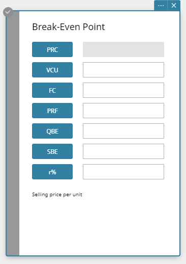
7-12-1. Break-Even Point Fields
The following fields appear on the Break-Even Point calculation.
| Field | Description |
|---|---|
| PRC | Selling price per unit |
| VCU | Variable cost per unit |
| FC | Fixed costs |
| PRF | Amount of profit realized |
| QBE | Number of units to be sold |
| SBE | Amount that must be obtained from sales to break even |
| $r$% | Proportion of sales amount retained as a profit (as a percent) |
7-12-2. Calculation Formulas
・Profit (Profit Amount/Ratio Setting: Amount (PRF))
$ SBE=\cfrac{FC+PRF}{PRC-VCU}\times{PRC} $
・Profit Ratio (Profit Amount/Ratio Setting: Ratio (r%))
$ SBE=\cfrac{FC}{PRC\times\left(1-\cfrac{r\%}{100}\right)-VCU}\times{PRC} $
7-13. Margin of Safety
Margin of Safety lets you calculate how much sales can be reduced before losses are incurred.
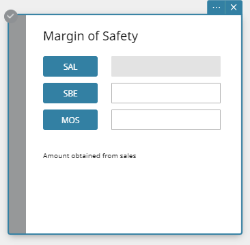
7-13-1. Margin of Safety Fields
The following fields appear on the Margin of Safety calculation.
| Field | Description |
|---|---|
| SAL | Amount obtained from sales |
| SBE | Break-even sales (amount that must be obtained from sales to break even) |
| MOS | Margin of safety (portion of sales amount above break-even point) |
7-13-2. Calculation Formulas
7-14. Operating Leverage
Operating Leverage lets you calculate the degree of change in net earnings arising from a change in sales amount.
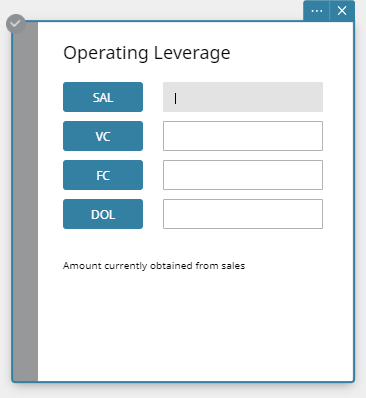
7-14-1. Operating Leverage Fields
The following fields appear on the Operating Leverage calculation.
| Field | Description |
|---|---|
| SAL | Amount currently obtained from sales |
| VC | Variable cost for this level of production |
| FC | Fixed costs |
| DOL | Degree of operating leverage |
7-14-2. Calculation Formulas
7-15. Financial Leverage
Financial Leverage lets you calculate the degree of change in net earnings arising from a change in interest paid.

7-15-1. Financial Leverage Fields
The following fields appear on the Financial Leverage calculation.
| Field | Description |
|---|---|
| EBIT | Earnings before interest and taxes |
| INT | Interest to be paid to bondholders |
| DFL | Degree of financial leverage |
7-15-2. Calculation Formulas
7-16. Combined Leverage
Combined Leverage lets you calculate the combined effects of operation and financial leverages.
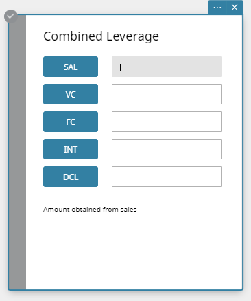
7-16-1. Combined Leverage Fields
The following fields appear on the Combined Leverage calculation.
| Field | Description |
|---|---|
| SAL | Amount obtained from sales |
| VC | Variable cost for this level of production |
| FC | Fixed costs |
| INT | Interest to be paid to bondholders |
| DCL | Degree of combined leverage |
7-16-2. Calculation Formulas
7-17. Quantity Conversion
Quantity Conversion lets you calculate the number of items sold, selling price, or sales amount given the other two values. It also lets you calculate the number of items manufactured, unit variable cost, or total variable cost given the other two values.
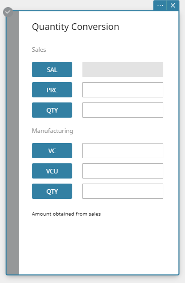
7-17-1. Quantity Conversion Fields
The following fields appear on the Combined Leverage calculation.
| Field | Description |
|---|---|
| SAL | Amount obtained from sales |
| PRC | Selling price per unit |
| QTY | Number of units sold |
| VC | Variable cost for this level of production |
| VCU | Variable cost per unit |
| QTY | Number of units manufactured |
7-17-2. Calculation Formulas
\( VC=VCU\times{QTY} \)