7. Functions
7-1. Graph Analysis Functions
| Trace | |
|---|---|
| Clicking a graph line to display the coordinates at that point. You can also drag the point along the graph line. | 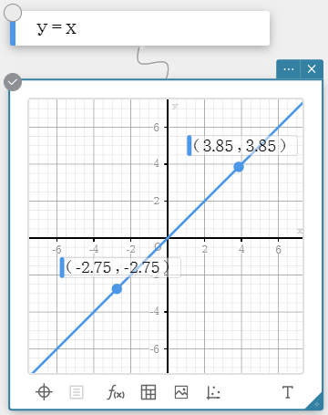 |
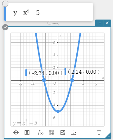
| Root (x-Intercept) | |
| Determines the root of a graph, and displays the point where the graph intercepts the X-axis. Click a point to show its coordinates. |
 |
| Min | |
| Determines the minimum value of a graph and displays a point at the minimum value. Click the point to show its coordinates. | 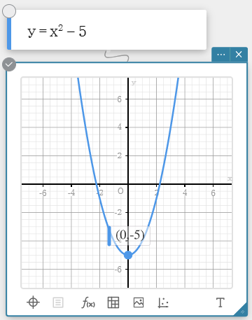 |
| Max | |
| Determines the maximum value of a graph and displays a point at the maximum value. Click the point to show its coordinates. | 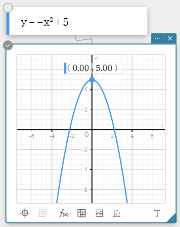 |
| y-Intercept | |
| Determines an x-coordinate value for a y-coordinate on a graph. Displays the point where the graph intercepts the Y-axis. Click the point to show its coordinates. | 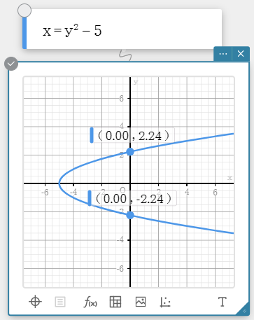 |
| Intersection | |
| Determines the points of intersection of two graphs and displays them. Click a point to show its coordinates. |
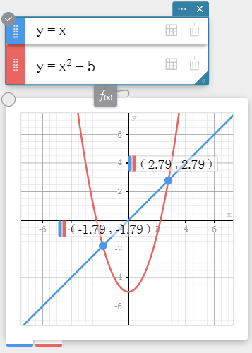 |
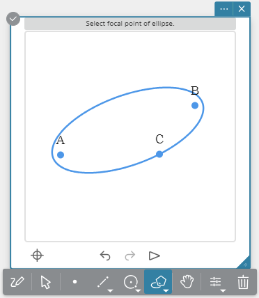
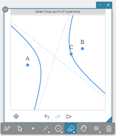
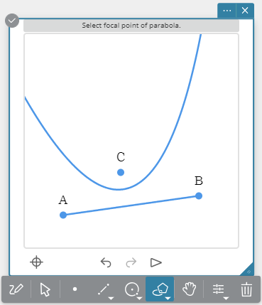
| Focus | |
| Determines the focus of a parabolic graph, elliptic graph, or hyperbolic curve graph. Drawing one of these types of graph causes the focus to be displayed. Click the point to show its coordinates. | 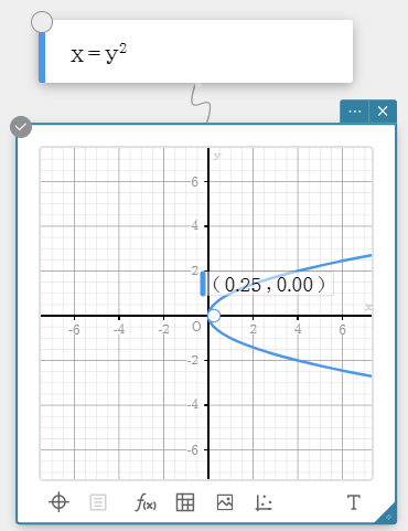 |
| Vertex | |
| Determines the vertex of a parabolic graph, elliptic graph, or hyperbolic curve graph. Drawing one of these types of graph causes the vertex to be displayed. Click the point to show its coordinates. | 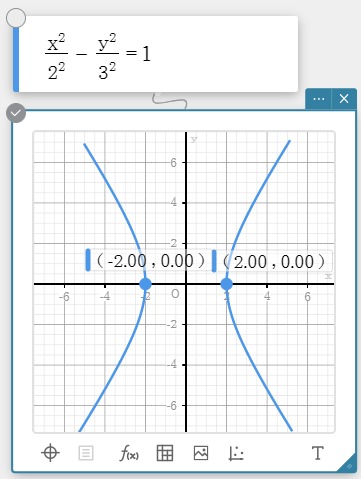 |
| Directrix | |
| Draws the directrix of a parabolic graph. Drawing a parabolic graph displays its directrix. Click the directrix to show its x-value and y-value. | 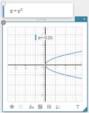 |
| Symmetry | |
| Draws the axis of symmetry of a parabolic graph. Drawing a parabolic graph displays its axis of symmetry. Click the axis of symmetry to show its x-value and y-value. | 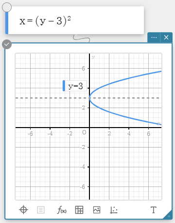 |
| Latus Rectum Length | |
| Determines the length of the latus rectum of a parabolic graph. Drawing a parabolic graph displays the length of it latus rectum. | 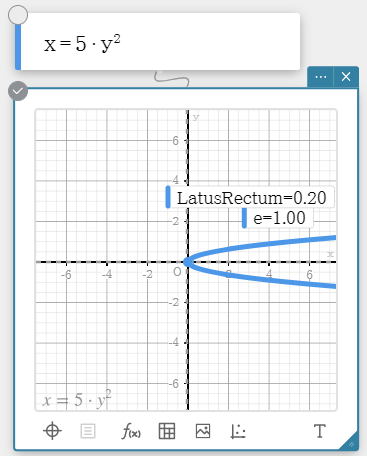 |
| Center | |
| Determines the center of a circle graph, elliptic graph, or hyperbolic curve graph. Drawing one of these types of graph causes the center to be displayed. Click the point to show its coordinates. | 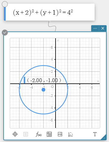 |
| Radius | |
| Determines the radius of a circle graph. Drawing a circle graph displays its radius. Click the radius to show its length ($r=$). | 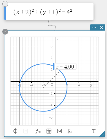 |
| Asympotes | |
| Draws the asympotes of a hyperbolic curve graph. Drawing a hyperbolic curve graph displays its asympotes. Click an asympote to show its equation. | 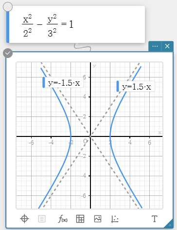 |
| Eccentricity | |
| Determines the eccentricity of a parabolic graph, elliptic graph, or hyperbolic curve graph. Drawing one of these types of graph causes the eccentricity ($e=$) to be displayed. | 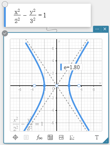 |
7-2. Statistical Calculations and Graphs
| One-Variable | |
|---|---|
|
This displays the calculation results of single-variable statistics. $x ̅$ ... sample mean $\Sigma x$ ... sum of data $\Sigma x^2$ ... sum of squares $\sigma x$ ... population standard deviation $Sx$ ... sample standard deviation $n$ ... sample size $minX$ ... minimum $Q1$ ... first quartile $Med$ .... median $Q3$ ... third quartile $maxX$ ... maximum $Mode$ ... mode $ModeN$ ... number of data mode items $ModeF$ ... data mode frequency When $Mode$ has multiple solutions, they are all displayed. |
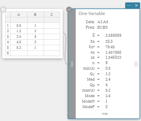 |
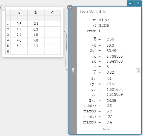
| Two-Variable | |
|
This displays the calculation results of paired-variable statistics. $x ̅$ ... sample mean $\Sigma x$ ... sum of data $\Sigma x^2$ ... sum of squares $\sigma x$ ... population standard deviation $Sx$ ... sample standard deviation $n$ ... sample size $y ̅$ ... sample mean $\Sigma y$ ... sum of data $\Sigma y^2$ ............. sum of squares $\sigma y$ ... population standard deviation $Sy$ ... sample standard deviation $\Sigma xy$ ... sum of the products XList and YList data $minX$ ... minimum $maxX$ ... maximum $minY$... minimum $maxY$ ... maximum |
 |
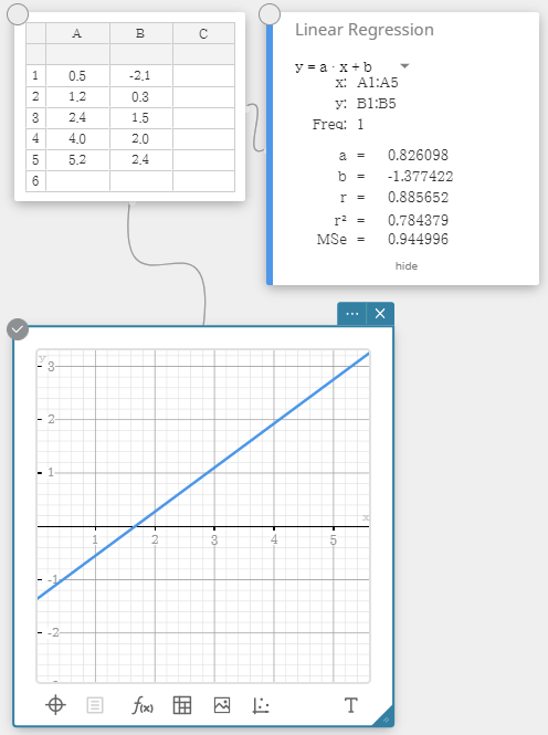
| Linear Regression | |
|
Linear regression uses the method of least squares to determine the equation that best fits your data points, and returns values for the slope and y-intercept. The graphic representation of this relationship is a linear regression graph. $y = ax + b$ $a$ ... regression coefficient (slope) $b$ ... regression constant term (y-intercept) $r$ .... correlation coefficient $r^2$ ... coefficient of determination $MSe$ ... mean square error |
 |
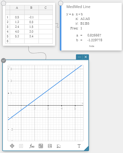
| MedMed Regression | |
|
When you suspect that the data contains extreme values, you should use the Med-Med graph (which is based on medians) in place of the linear regression graph. Med-Med graph is similar to the linear regression graph, but it also minimizes the effects of extreme values. $y = ax + b$ $a$ ... regression coefficient (slope) $b$ ... regression constant term (y-intercept) |
 |
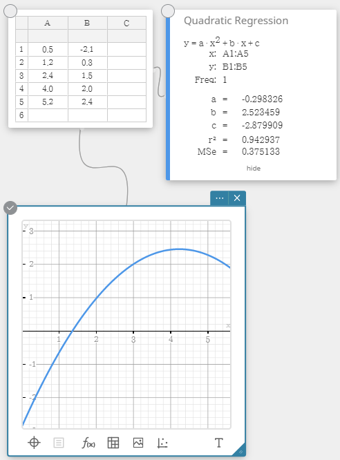
| Quadratic Regression | |
|
Quadratic regression graph uses the method of least squares to draw a curve that passes the vicinity of as many data points as possible. This graph can be expressed as quadratic regression expression. $y = ax2 + bx + c$ $a$ ... regression second coefficient $b$ ... regression first coefficient $c$ ... regression constant term (y-intercept) $r^2$ ... coefficient of determination $MSe$ ... mean square error |
 |
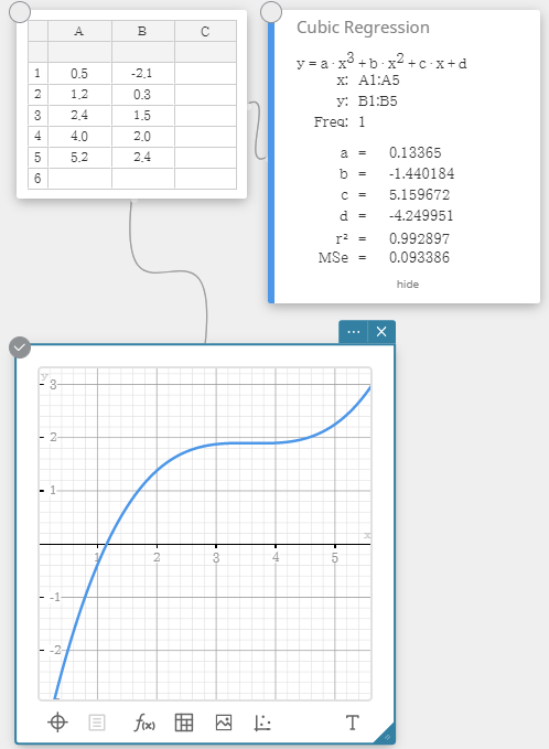
| Cubic Regression | |
|
Cubic regression graph uses the method of least squares to draw a curve that passes the vicinity of as many data points as possible. This graph can be expressed as cubic regression expression. $y = ax3 + bx2 + cx + d$ $a$ ... regression third coefficient $b$ ... regression second coefficient $c$ ... regression first coefficient $d$ ... regression constant term (y-intercept) $r^2$ ... coefficient of determination $MSe$ ... mean square error |
 |
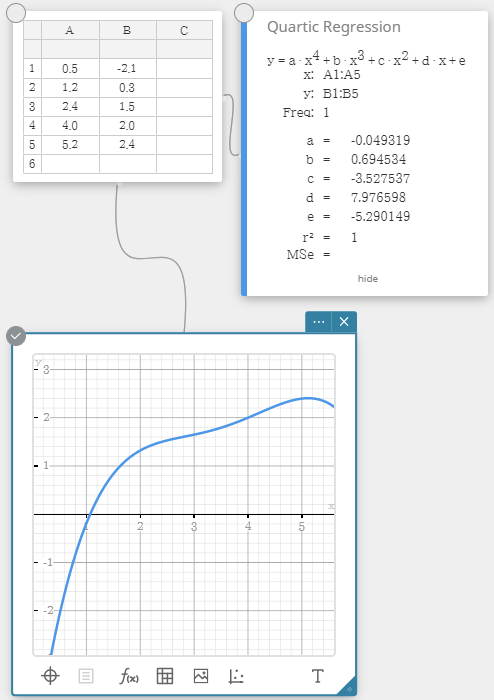
| Quartic Regression | |
|
Quartic regression graph uses the method of least squares to draw a curve that passes the vicinity of as many data points as possible. This graph can be expressed as quartic regression expression. $y = ax4 + bx3 + cx2 + dx + e$ $a$ ... regression fourth coefficient $b$ ... regression third coefficient $c$ ... regression second coefficient $d$ ... regression first coefficient $e$ ... regression constant term (y-intercept) $r^2$ ... coefficient of determination $MSe$ ... mean square error |
 |
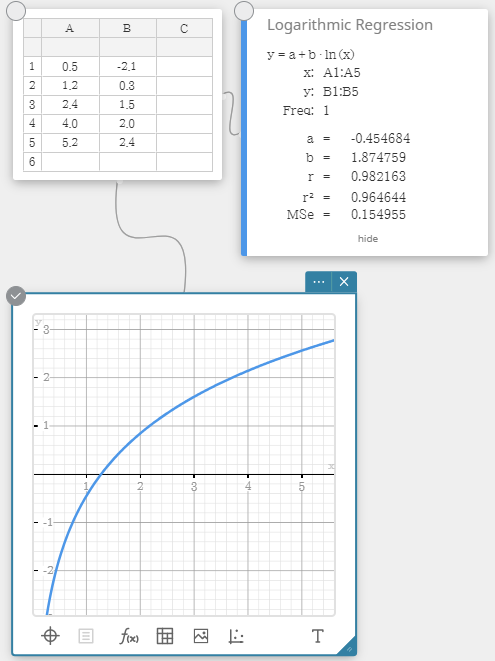
| Logarithmic Regression | |
|
Logarithmic regression expresses $y$ as a logarithmic function of $x$. The normal logarithmic regression formula is $y=a+b \cdot ln(x)$. If we say that $X=ln(x)$, then this formula corresponds to the linear regression formula $y=a+b \cdot X$. $y = a + b \cdot ln\ x$ $a$ ... regression constant term $b$ ... regression coefficient $r$ .... correlation coefficient $r^2$ ... coefficient of determination $MSe$ ... mean square error |
 |
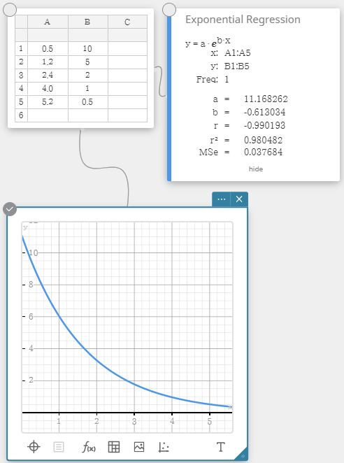
| Exponential Regression | |
|
Exponential regression can be used when $y$ is proportional to the exponential function of $x$. The normal exponential regression formula is $y=a \cdot e^{b \cdot x}$. If we obtain the logarithms of both sides, we get $ln(y)=ln(a)+b \cdot x$. Next, if we say that $Y=ln(y)$ and $A=In(a)$, the formula corresponds to the linear regression formula $Y=A+b \cdot x$. $y = a \cdot e^{bx}$ $a$ ... regression coefficient $b$ ... regression constant term $r$ .... correlation coefficient $r^2$ ... coefficient of determination $MSe$ ... mean square error |
 |
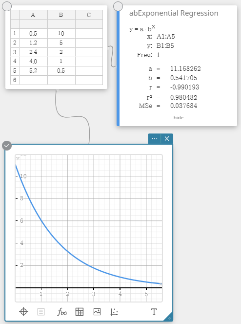
| abExponential Regression | |
|
Exponential regression can be used when $y$ is proportional to the exponential function of $x$. The normal exponential regression formula in this case is $y=a \cdot b^x$. If we take the natural logarithms of both sides, we get $ln(y)=ln(a)+(ln(b)) \cdot x$. Next, if we say that $Y=ln(y)$, $A=ln(a)$ and $B=ln(b)$, the formula corresponds to the linear regression formula $Y=A+B \cdot x$. $y = a \cdot b^x$ $a$ ... regression constant term $b$ ... regression coefficient $r$ .... correlation coefficient $r^2$ ... coefficient of determination $MSe$ ... mean square error |
 |
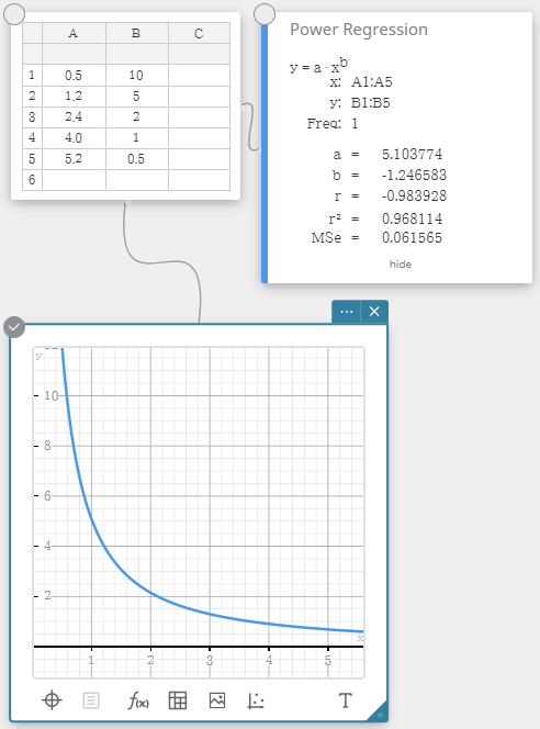
| Power Regression | |
|
Power regression can be used when $y$ is proportional to the power of $x$. The normal power regression formula is $y=a \cdot x^b$. If we obtain the logarithms of both sides, we get $ln(y)=ln(a)+b \cdot ln(x)$. Next, if we say that $X=ln(x)$, $Y=ln(y)$, and $A=ln(a)$, the formula corresponds to the linear regression formula $Y=A+b \cdot X$. $y = a \cdot x^b$ $a$ ... regression coefficient $b$ ... regression power $r$ .... correlation coefficient $r^2$ ... coefficient of determination $MSe$ ... mean square error |
 |
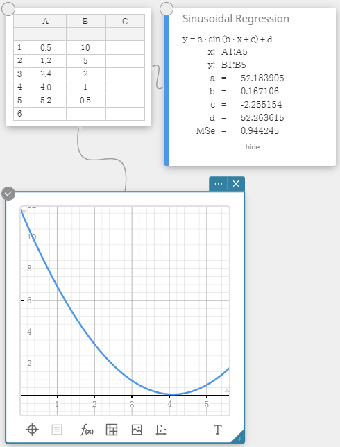
| Sinusoidal Regression | |
|
Sinusoidal regression is best for data that repeats at a regular fixed interval over time. $y = a \cdot sin( bx + c ) + d$ $a$, $b$, $c$, $d$ ... regression coefficient $MSe$ ... mean square error |
 |
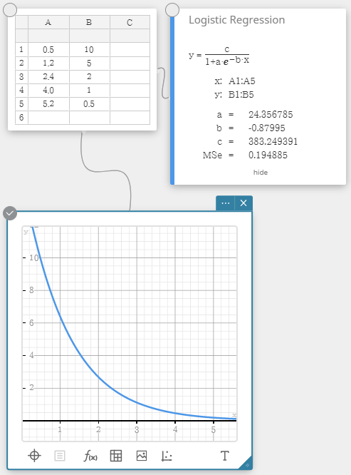
| Logistic Regression | |
|
Logistic regression is best for data whose values continually increase over time, until a saturation point is reached. $y=\cfrac{c}{1+ae^{-bx}}$ $a$, $b$, $c$ ... regression coefficient $MSe$ ... mean square error |
 |
| Scatter Plot | |
| This plot compares the data accumulated ratio with a normal distribution accumulated ratio. If the scatter plot is close to a straight line, then the data is approximately normal. A departure from the straight line indicates a departure from normality. | 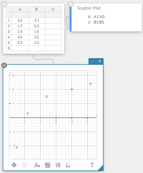 |
| Box & Whisker Plot | |
| This type of graph lets you see how a large number of data items are grouped within specific ranges. A box encloses all the data in an area from the first quartile ($Q1$) to the third quartile ($Q3$), with a line drawn at the median ($Med$). Lines (called whiskers) extend from either end of the box up to the minimum ($minX$) and maximum ($maxX$) of the data. | 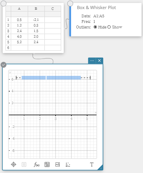 |
| Histogram | |
| A histogram shows the frequency (frequency distribution) of each data class as a rectangular bar. Classes are on the horizontal axis, while frequency is on the vertical axis. You can change the start value ($HStart$) and step value ($HStep$) of the histogram, if you want. | 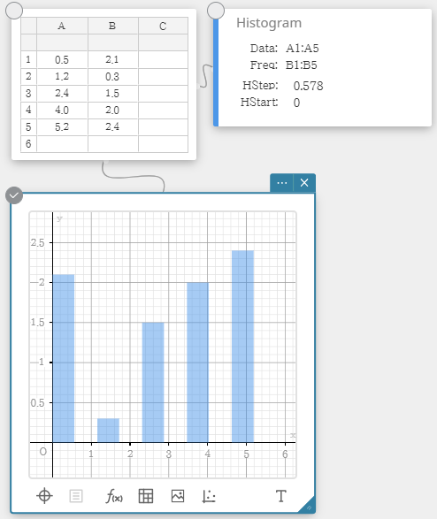 |
| Pie Chart | |
| You can draw a circle graph based on the data in a specific list. | 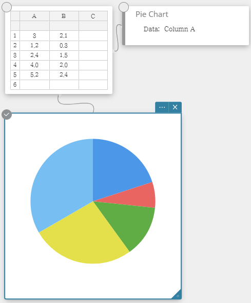 |
| Dot Plot | |
| The values in Column A (horizontal axis) represents bin numbers, while the values in Column B (vertical axis) represent the data point count in each bin. A dot is plotted for each data point in a bin. | 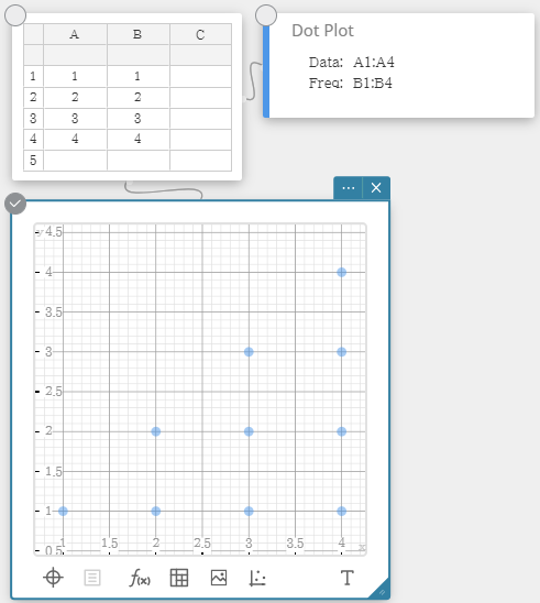 |
| Normal CD | |
| Calculates the cumulative probability of a normal distribution between a lower bound and an upper bound. | 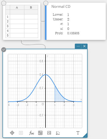 |
7-3. Drawable Figures
 Drawing Drawing |
|
|---|---|
| This tool can be used for freehand point plotting, or drawing of a line segment, polyline, polygon, or circle. |  |
 Point Point |
|
| Click the location where you want to plot a point. |  |
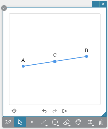
 Segment Segment |
|
|
1. Click the location you want specify as the line segment start point. 2. Click the location you want specify as the line segment end point. ・This will draw a line segment between the two specified points. |
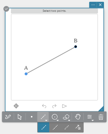 |
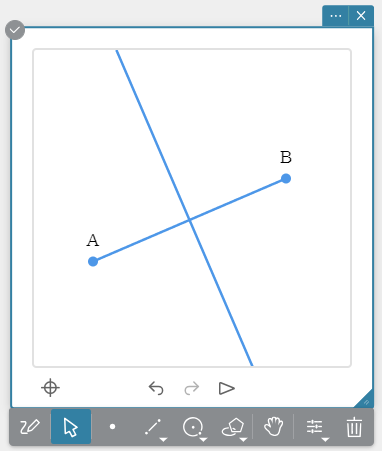
 Line Line |
|
|
1. Click any location. 2. Click another location. ・This will draw a straight line that passes between the two points. |
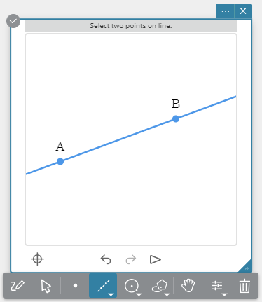 |
 Ray Ray |
|
|
1. Click any location. 2. Click another location. ・This will draw a ray that starts from the first point you specified and passes through the second point. |
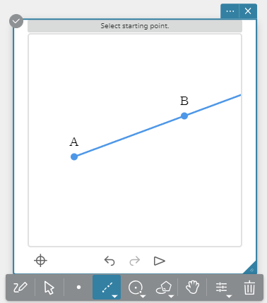 |
 Vector Vector |
|
|
1. Click the location you want specify as the vector start point. 2. Click the location you want specify as the vector end point. |
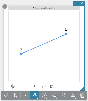 |
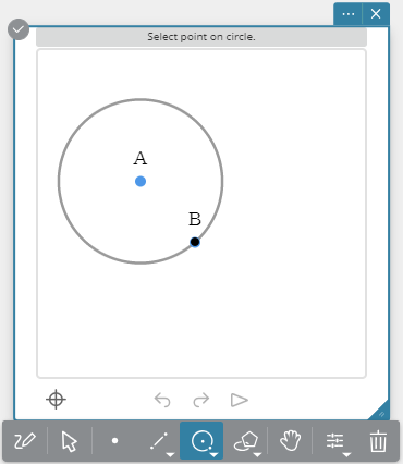
 Circle Circle |
|
|
1. Click the location you want to specify as the circle center point. 2. Click the location you want to specify as one point on the circle periphery. ・The radius of the circle will be distance between the two points you specify. |
 |
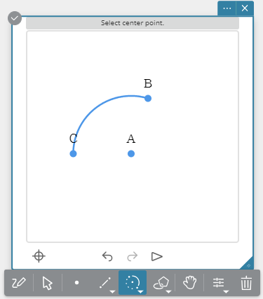
 Arc Arc |
|
|
1. Click the location you want to specify as the circle center point. 2. Click the location you want to specify as the arc start point. 3. Click the location you want to specify as the arc end point. ・An arc will be drawn from the start point to the end point, in a counterclockwise direction. |
 |
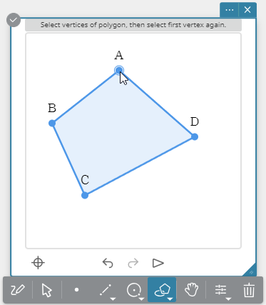
 Polygon Polygon |
|
|
1. Click the location you want to specify as a vertex of the polygon. 2. Click the locations you want to specify as the other vertices of the polygon. 3. To complete the polygon, click the location of the first vertex. |
 |
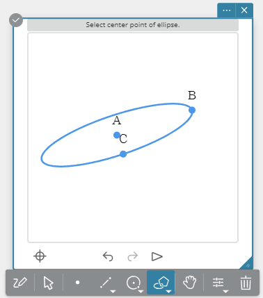
 Ellipse (Axes) Ellipse (Axes) |
|
|
1. Click the location you want to specify as the center point. 2. Click the location you want specify as the minor axis (closest point to the center point). 3. Click the location you want specify as the major axis (furthest point from the center point). ・You can also perform the above steps 2 and 3 in reverse sequence. |
 |
 Ellipse (Foci) Ellipse (Foci) |
|
|
1. Click two locations you want to specify as the foci. 2. Click the location you want to specify as any point on the ellipse periphery. |
 |
 Hyperbola Hyperbola |
|
|
1. Click two locations you want to specify as the foci. 2. Click the location you want to specify as any point on the hyperbolic curve. |
 |
 Parabola Parabola |
|
|
1. Draw the line segment, straight line, ray, or vector to be used as the directrix of the parabola. 2. On the Object menu, click [Parabola]. 3. Click the location you want to specify as the focus. 4. Click the directrix you drew in step 1. |
 |
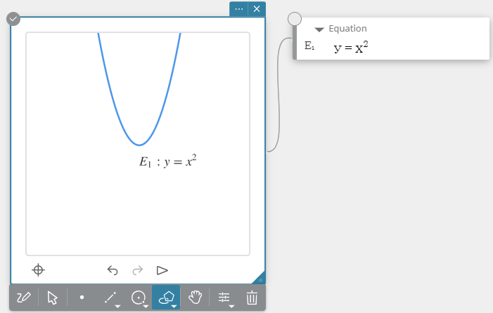
 Function Function |
|
|
1. On the Object menu, click [Function]. ・This displays an Equation Sticky Note. 2. Input a function into the Equation Sticky Note, and then click [EXE] on the soft keyboard. |
 |
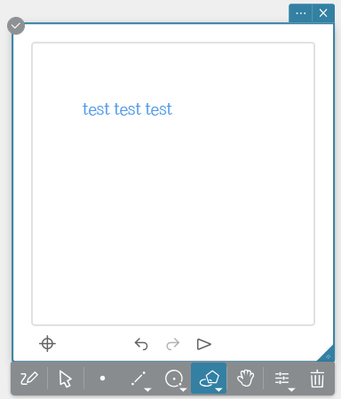
 Text Text |
|
|
1. On the Object menu, click [Text]. 2. Click the location where you want to insert text. ・This will display a text input box. 3. Input the text and then press [Enter] on your computer keyboard. |
 |
7-4. Adjustment Functions
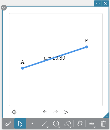
 Length Length |
|
|---|---|
|
1. Draw a line segment. 2. Select the line segment. 3. Click [Length]. ・The current length of the line segment is shown at the top of the Geometry Sticky Note. 4. Change the line segment length and then press [Enter] on your computer keyboard. Note ・This operation can be executed while a line segment, a vector, or one side of a polygon is selected. |
 |
 Congruent Congruent |
|
|
1. Draw a triangle. 2. Select two sides. 3. Click [Congruent]. Note ・The length of the second line you select is changed to match the length of the first line you selected in step 2. ・This operation can be executed while any two of the following items (two of the same type, or one each of different types) are selected: line segment, vector, or one side of a polygon. |
 |
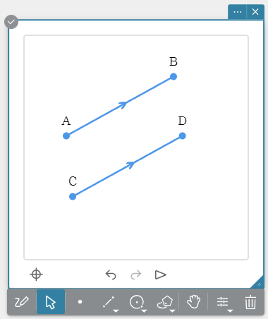
 Parallel Parallel |
|
|
1. Draw two line segments. 2. Select the two line segments. 3. Click [Parallel]. Note ・The orientation of the second line you select is changed to match the orientation of the first line you selected in step 2. ・An arrow symbol (>) will appear on both lines when they are parallel with each other. ・Any two of the following items (two of the same type, or one each of different types) can be selected and made parallel with each other: line segment, straight line, ray, vector, or one side of a polygon. |
 |
 Perpendicular Perpendicular |
|
|
1. Draw two line segments. 2. Select the two line segments. 3. Click [Perpendicular]. Note ・The orientation of the second line you select is changed to make it perpendicular with the first line you selected in step 2. ・Any two of the following items (two of the same type, or one each of different types) can be selected and made perpendicular with each other: line segment, straight line, ray, vector, or one side of a polygon. |
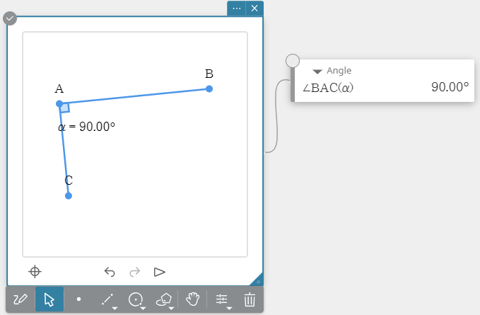 |
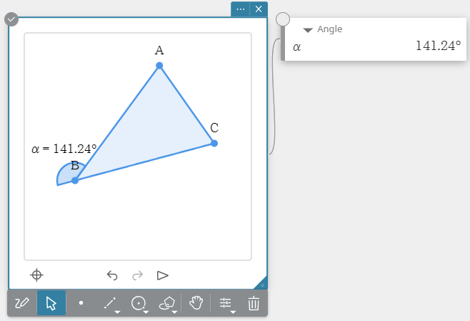
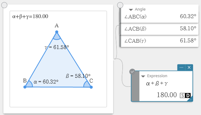
 Angle Angle |
|
|
1. Draw a triangle. 2. Select two sides. 3. Click [Angle]. ・The current angle is shown at the top of the Geometry Sticky Note. 4. Change the angle and then press [Enter] on your computer keyboard. Note ・The angle of the second line you select is changed based on the line segment you selected in step 2. ・This operation can be executed while any two of the following items (two of the same type, or one each of different types) are selected: line segment, straight line, ray, vector, or one side of a polygon. |
 |
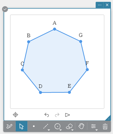
 Regular Polygon Regular Polygon |
|
|
1. Draw an n-gon. 2. Select the n-gon. 3. Click [Regular Polygon]. ・This changes the figure to a regular n-gon. |
 |
7-5. Measurement Functions
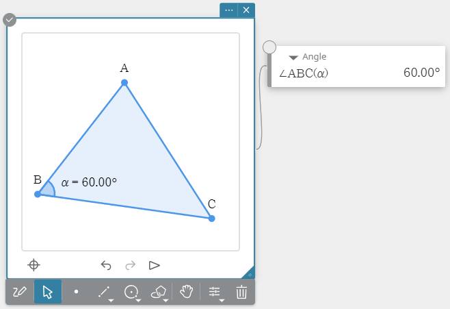
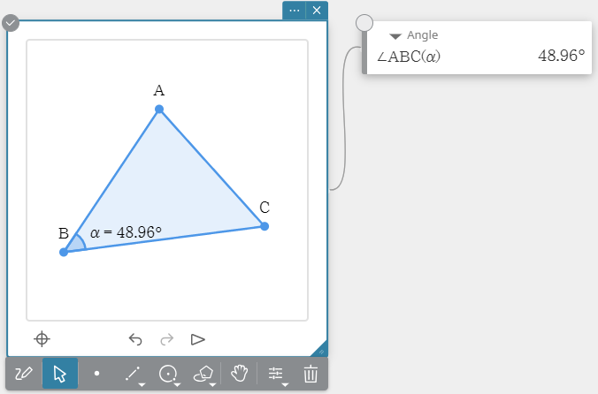
 Angle Angle |
|
|---|---|
|
1. Draw a triangle. 2. Select two sides. 3. Click [Angle]. Note ・This operation can be executed while any two of the following items (two of the same type, or one each of different types) are selected: line segment, straight line, ray, vector, or one side of a polygon. |
 |
 Supplementary Angle Supplementary Angle |
|
|
1. Draw a triangle. 2. Select two sides. 3. Click [Supplementary Angle]. Note ・The position of the supplementary angle that is measured depends on sequence of the two sides you select in step 2. ・This operation can be executed while any two of the following items (two of the same type, or one each of different types) are selected: line segment, straight line, ray, vector, or one side of a polygon. |
 |
 Interior angle Interior angle |
|
|
1. Draw a regular n-polygon. 2. Select the regular n-polygon. 3. Click [Interior angle]. |
|
|
Exterior angle |
|
|
1. Draw a regular n-polygon. 2. Select the regular n-polygon. 3. Click [Exterior angle]. |
|
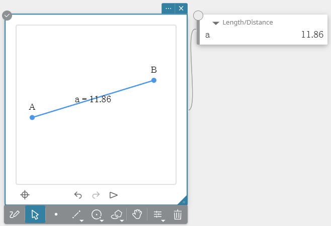
 Length/Distance Length/Distance |
|
|
1. Draw a line segment. 2. Select the line segment. 3. Click [Length/Distance]. Note ・This operation can be executed while any two points, a line segment, a vector, or one side of a polygon is selected. |
 |
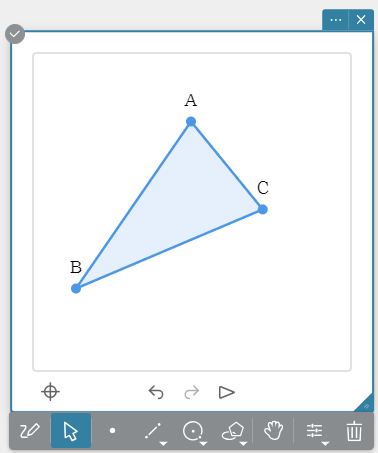
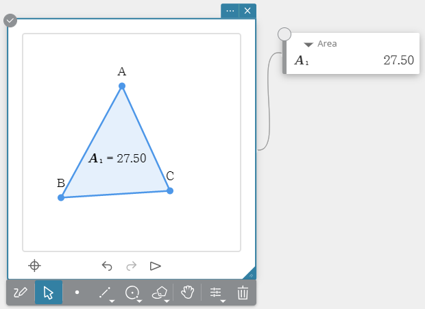
 Area Area |
|
|
1. Draw a triangle. 2. Select the triangle. 3. Click [Area]. Note ・This operation can be executed while a circle, ellipse, or polygon is selected. |
 |
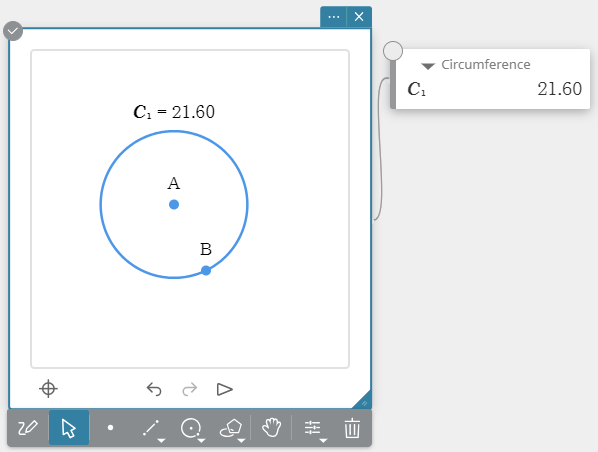
 Circumference/Perimeter Circumference/Perimeter |
|
|
1. Draw a circle. 2. Select the circle. 3. Click [Circumference/Perimeter]. Note ・This operation can be executed while a circle, ellipse, or polygon is selected. |
 |
 Radius Radius |
|
|
1. Draw a circle. 2. Select the circle. 3. Click [Radius]. |
 |
 Slope Slope |
|
|
1. Draw a line segment. 2. Select the line segment. 3. Click [Slope]. Note ・This operation can be executed while a line segment, straight line, ray, vector, or one side of a polygon is selected. |
 |
 Direction Direction |
|
|
1. Draw a line segment. 2. Select the line segment. 3. Click [Direction]. Note ・This operation can be executed while a line segment, straight line, ray, vector, or one side of a polygon is selected. |
 |
 Coordinates Coordinates |
|
|
1. Plot a point. 2. Select the point. 3. Click [Coordinates]. |
 |
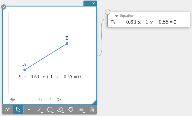
 Equation Equation |
|
|
1. Draw a line segment. 2. Select the line segment. 3. Click [Equation]. Note ・This operation can be executed while a line segment, straight line, ray, vector, circle, ellipse, or one side of a polygon is selected. |
 |
 Expression Expression |
|
|
1. Click [Expression]. 2. On the Expression Tab, input the expression. 3. On the soft keyboard, click [EXE]. |
 |
7-6. Construction Functions
 Prep. Bisector Prep. Bisector |
|
|---|---|
|
1. Draw a line segment. 2. Select the line segment. 3. Click [Prep. Bisector]. Note ・This operation can be executed while one line segment, one side of a polygon, or two points are selected. |
 |
 Perpendicular Perpendicular |
|
|
1. Draw a line segment and plot a point. 2. Select the line segment and point. 3. Click [Perpendicular]. ・This will draw a perpendicular to the selected line segment that passes through the selected point. Note ・This operation can be executed while a single line segment and single point, a single line and single point, a single ray and a single point, a single vector and a single point, or one side of a polygon and a single point are selected. |
 |
 Midpoint Midpoint |
|
|
1. Draw a line segment. 2. Select the line segment. 3. Click [Midpoint]. ・This will construct the midpoint of the line segment you selected. Note ・This operation can be executed while one line segment, one side of a polygon, or two points are selected. |
 |
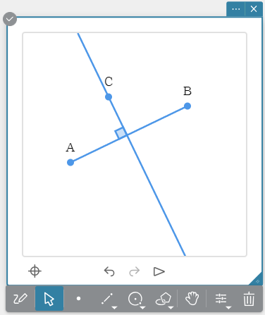
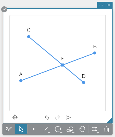
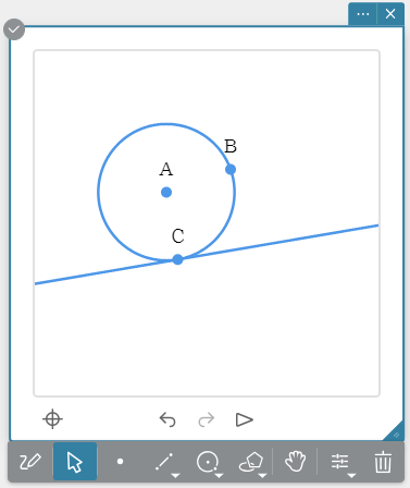
 Intersection Intersection |
|
|
1. Draw two intersecting line segments. 2. Select the two line segments. 3. Click [Intersection]. Note ・This operation can be executed while any two of the following items (two of the same type, or one each of different types) are selected: line segment, straight line, ray, vector, one side of a polygon, circle, arc, ellipse, hyperbolic curve, or parabola. |
 |
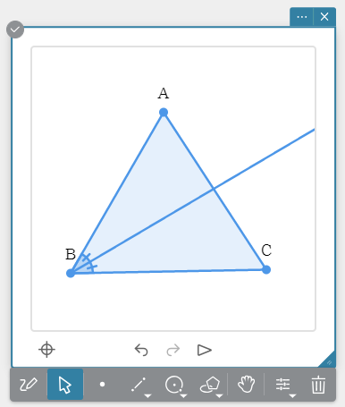
 Angle Bisector Angle Bisector |
|
|
1. Draw a triangle. 2. Select two sides. 3. Click [Angle Bisector]. Note ・This operation can be executed while any two of the following items (two of the same type, or one each of different types) are selected: line segment, straight line, ray, vector, or one side of a polygon. |
 |
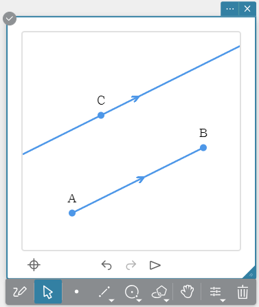
 Parallel Parallel |
|
|
1. Draw a line segment and plot a point. 2. Select the line segment and point. 3. Click [Parallel]. Note ・Constructing parallel lines will cause arrow symbols (>) to appear on the two lines to indicate that they are parallel with each other. ・This operation can be executed while any combination of the objects below is selected.
- A single line segment and a single point, a single line and a single point, a single ray and a single point, a single vector and a single point
- One side of a polygon and a single point - A pair of lines (straight line, ray, vector, one side of a polygon, etc.) |
 |
 Tangent to Curve Tangent to Curve |
|
|
1. Draw a circle. 2. Select the circle. 3. Click [Tangent to Curve]. ・Starting with a point on the curve, this function constructs a straight line that passes through that point. ・The position of the straight line can be changed by dragging the point. Note ・This operation can be executed while a circle, ellipse, or function graph is selected. |
 |
 Regular n-polygon Regular n-polygon |
|
|
1. Draw a line segment. 2. Select the line segment. 3. Click [Regular n-polygon]. 4. Input the number of angles in the regular polygon you want to create in the Regular n-polygon Sticky Note. Note ・This will construct a regular polygon with the selected line segment as one side. |
|
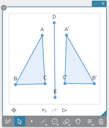
 Reflection Reflection |
|
|
1. Draw the figure that will be the basis of the reflection symmetry mapping and the line segment that will be the line of symmetry. 2. Select the figure that is the basis of the reflection symmetry mapping. 3. Click [Reflection]. 4. Select the line segment to use as axis of symmetry. ・This creates a reflection symmetry mapping of the original figure with the selected line segments as the axis of symmetry. Note ・You can specify a line segment, line, ray, or one side of a polygon as an axis of symmetry. |
 |
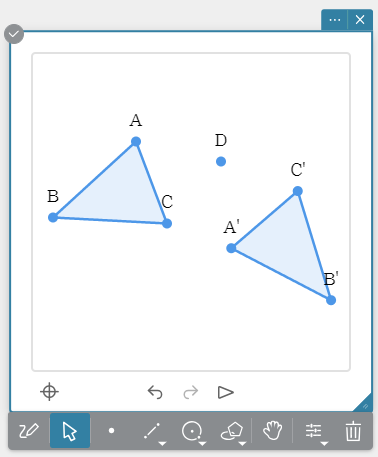
 Rotation Rotation |
|
|
1. Draw a figure that will be the basis of the rotation mapping and plot a point as the rotation center. 2. Select the figure that will be the basis of the rotation mapping. 3. Click [Rotation]. 4. Select the rotation center point. 5. Input the angle of rotation (counterclockwise) as a degree value. ・This will create a figure that is the rotated version of the original figure. Note ・Inputting a variable for the rotation angle will display a slider. You can use the slider to view rotation of the figure as the variable value changes. |
 |
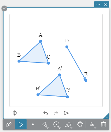
 Translation Translation |
|
|
1. Draw the figure that will be the basis of the translation mapping. 2. Select the figure. 3. Click [Translation]. 4. Input a value to specify the amount of movement. ・This will create a mapping that is the translated version of the original figure. Note ・Inputting a variable for the amount of movement will display a slider. You can use the slider to view translation of the figure as the variable value changes.Inputting a variable for the amount of movement will display a slider. You can use the slider to view translation of the figure as the variable value changes. |
 |
 Dilation Dilation |
|
|
1. Draw a figure to be dilated. 2. Plot a point as the dilation center. 3. Select the figure to be dilated. 4. Click [Dilation]. 5. Input the dilation factor. ・This will draw a resized version of the original object. Note ・Inputting a variable for the dilation factor will display a slider. You can use the slider to view dilation of the figure as the variable value changes. |
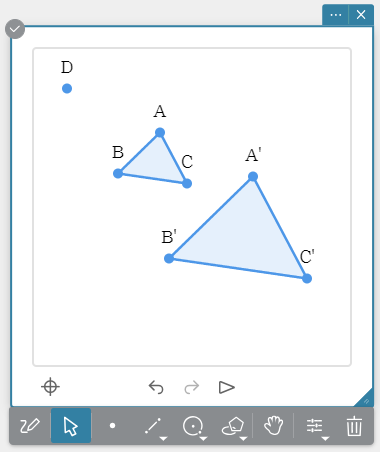 |
|
Compass |
|
|
1. Draw a line segment. 2. Select the line segment. 3. Click [Compass]. ・This will construct a circle whose radius is the length of the selected line segment. Note ・You can execute construction of a circle while one line segment or two points are selected. ・Changing the length of a line segment will change the size of the circle linked with it. |
|