4. Statistical Calculations
- 4-1. Basic Statistical Calculation Operations
- 4-2. Editing Statistical Data Values
- 4-3. Selecting Data Values for Statistical Calculation
- 4-4. Performing 1-variable Statistical Calculations
- 4-5. Drawing a Regression Graph
- 4-6. Drawing a Histogram
- 4-7. Drawing a Box-and-whisker Diagram
- 4-8. Drawing a Circle Graph
- 4-9. Scatter Plot Operations
- 4-10. Performing a One-Sample Z-Test
- 4-11. Statistical Calculations and Graphs
4-1. Basic Statistical Calculation Operations
4-1-1. Inputting Values into a Statistical Data Sticky Note
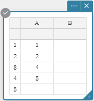
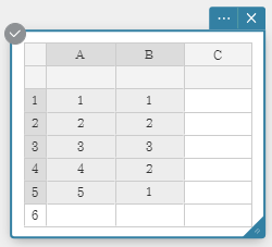
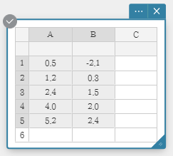
In the example shown in this section, the data values in the table below are input into cells A1 through B5 of a Statistical Data Sticky Note.
| A | B | |
| 1 | $0.5$ | $-2.1$ |
| 2 | $1.2$ | $0.3$ |
| 3 | $2.4$ | $1.5$ |
| 4 | $4.0$ | $2.0$ |
| 5 | $5.2$ | $2.4$ |
1. Click anywhere on the Paper.
• This displays the Sticky Note menu.

2. Click  .
.
• This displays a Statistical Data Sticky Note.

• Cell A1 becomes selected for input at this time.
3. Input $0.5$ into cell A1 and then press [Enter].
• Cell A2 becomes selected for input.
4. Input $1.2$ into cell A2 and then press [Enter].
• Cell A3 becomes selected for input. Similarly, input data up to cell A5.
5. Click cell B1.
• Cell B1 becomes selected for input.
6. Input $-2.1$ into cell B1 and then press [Enter]. This automatically creates column C. For more information, see the note below.
• Cell B2 becomes selected for input.
7. Input $0.3$ into cell B2 and then press [Enter].
• Cell B3 becomes selected for input. Similarly, input data up to cell B5.

Note
- Inputting a value into the rightmost column automatically adds a new column to the right of it.

- The cells under the column labels (A, B, C,...) can be used to input a list name for each column. For details, see "4-2-6. Assigning a Name to a List".
4-1-2. Selecting Data Values for Statistical Calculation
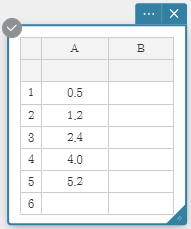
1. Use the procedure under "4-1-1. Inputting Values into a Statistical Data Sticky Note" to input data values.
| A | B | |
| 1 | $0.5$ | $-2.1$ |
| 2 | $1.2$ | $0.3$ |
| 3 | $2.4$ | $1.5$ |
| 4 | $4.0$ | $2.0$ |
| 5 | $5.2$ | $2.4$ |
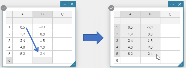
2. Use your computer mouse to drag from cell A1 to cell B5.
• This selects the range of cells from A1 through B5.
Note
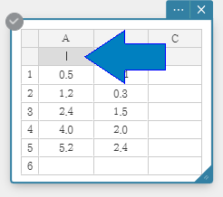
- You can select an entire column by clicking its column number.
- You can select an entire row by clicking its row number.
- You can click or drag across column numbers and use the data in those columns to draw a graph.
In this case, after drawing the graph you can also use the drop-down list of the Graph Sticky Note to select other column numbers and redraw the graph.
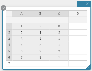
4-1-3. Performing Statistical Calculations
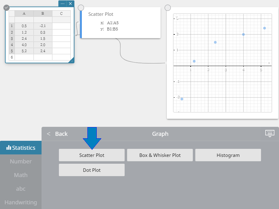
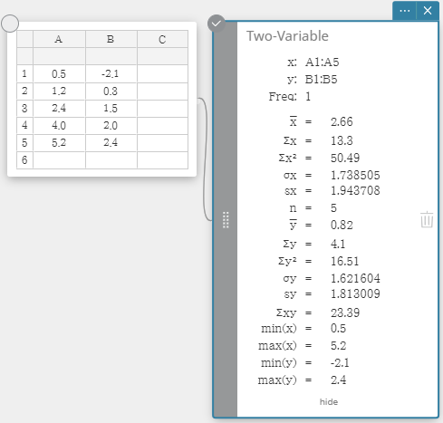
In this example, we perform two-variable statistical calculations and draw a scatter plot and a linear regression graph.
1. Input the data values in the table below, and then select all of the data.
|
|
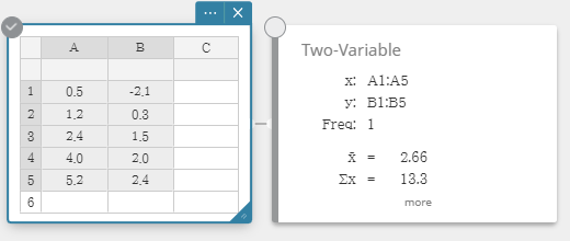
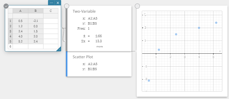
2. On the soft keyboard, click [Calculation] - [Two-Variable].

• This displays two-variable statistical calculation results.
3. On the soft keyboard, click  .
.

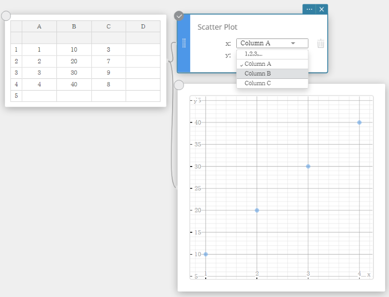
4. On the soft keyboard, click [Graph] - [Scatter Plot].
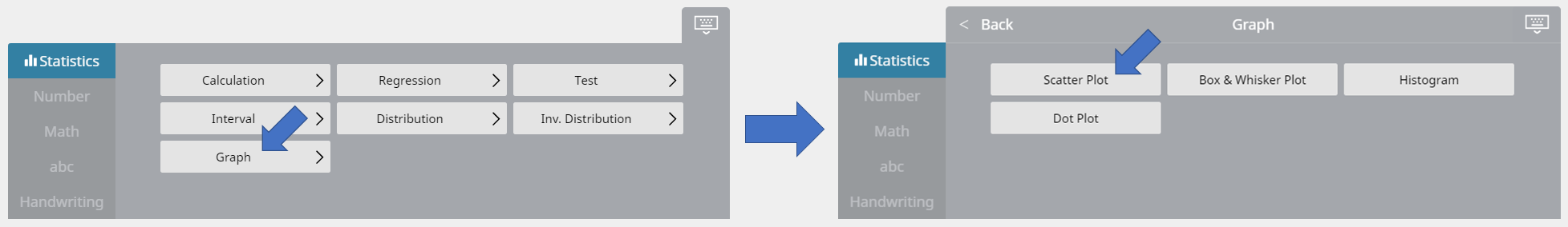
• This creates a Scatter Plot Sticky Note and draws a scatter plot on the Graph Sticky Note simultaneously.
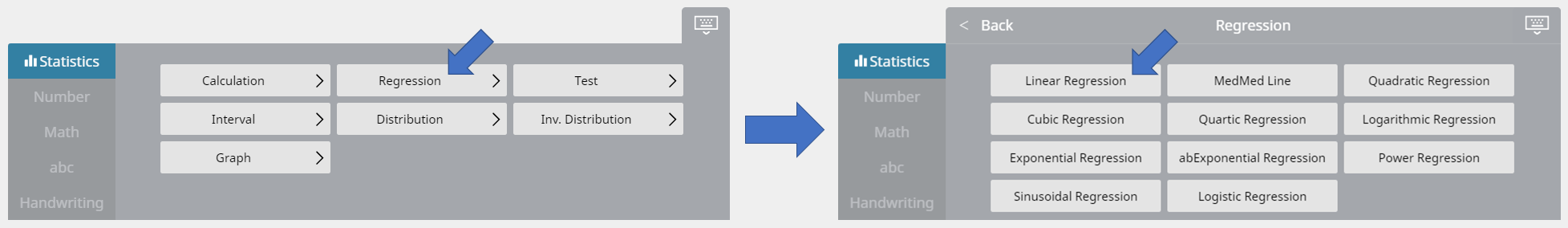
5. On the soft keyboard, click .
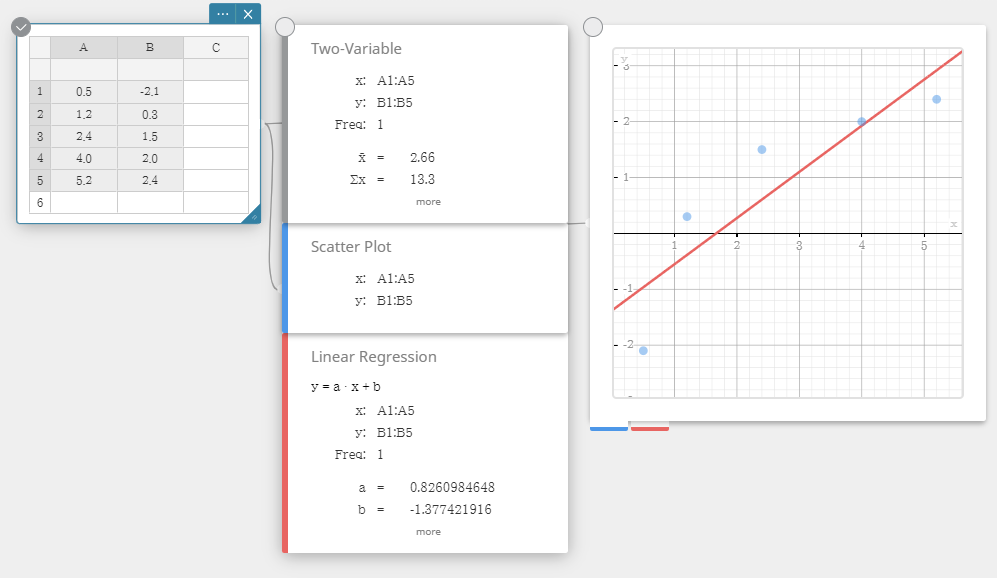
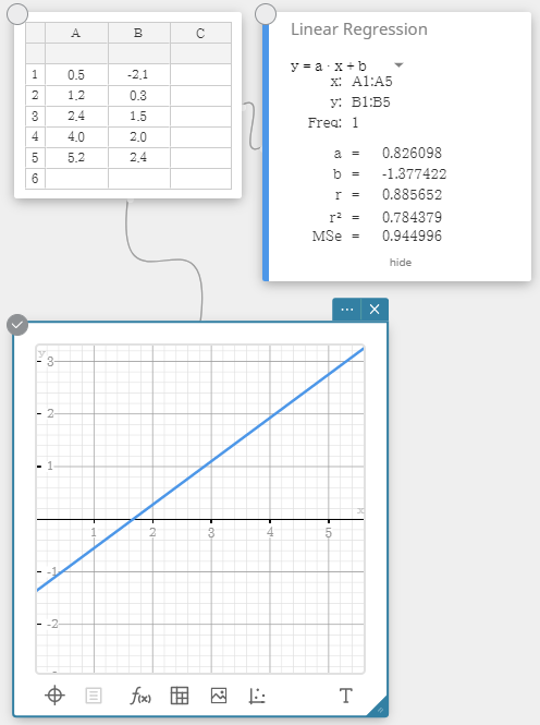
6. On the soft keyboard, click [Regression] - [Linear Regression].

• This creates a Linear Regression Sticky Note and draws a linear regression graph on the Graph Sticky Note simultaneously.
4-2. Editing Statistical Data Values
4-2-1. To correct data values
1. Click on the cell that contains the data value you want to correct.
2. Input the new data value and then press [Enter].
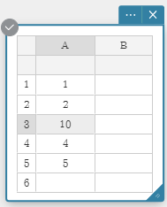
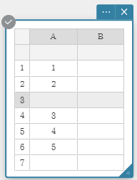
4-2-2. To insert a row
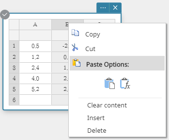
1. Right-click the number of the row where you want to insert a new row.
• This displays a menu.

2. Click [Insert] to insert the row.
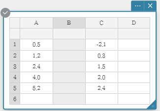
4-2-3. To insert a column
1. Right-click the header of the column where you want to insert a new column.
• This displays a menu.
2. Click [Insert] to insert the column.
4-2-4. To delete a row
1. Right-click the number of the row you want to delete.
• This displays a menu.

2. Click [Delete] to delete the row.
4-2-5. To delete a column
1. Right-click the header of the column you want to delete.
• This displays a menu.
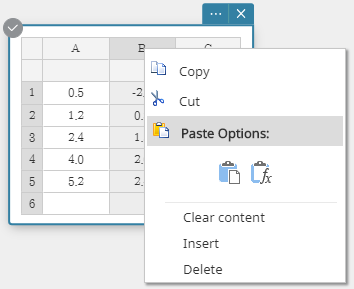
2. Click [Delete] to delete the column.
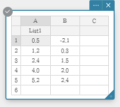
4-2-6. Assigning a Name to a List
Once you assign a name to a list, you can use the name in tests and other statistical calculations. List names are input into the cells below the column names.
Example: To assign the name "List1" to column A
1. Double-click the cell under A.
• This selects the cell for list name input.
2. Input the list name "List1" and then press [Enter].
• This assigns "List 1" as the list name of column A.
Note
• The following are the rules that apply to list names.
- - List names can be up to 8 bytes long.
- - The following characters are allowed in a list name: Upper-case and lower-case characters, subscript characters, numbers.
- - List names are case-sensitive. For example, each of the following is treated as a different list name: abc, Abc, aBc, ABC.
4-3. Selecting Data Values for Statistical Calculation
You can select a range of cells by dragging the mouse pointer across them.
Data Selection Examples
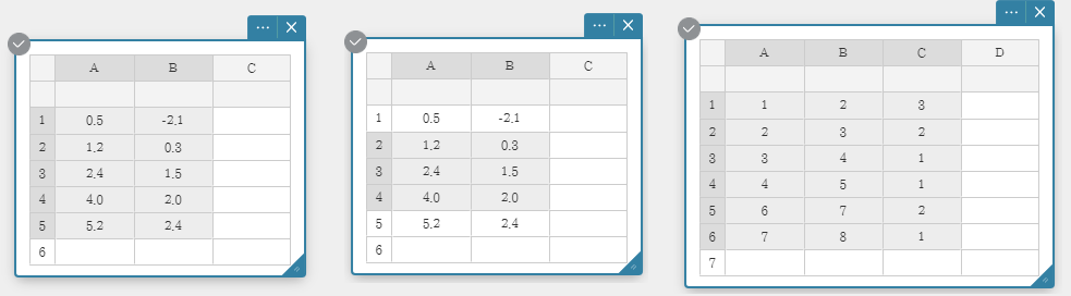
Note
- You can select an entire column by clicking its column number.
- You can select an entire row by clicking its row number.
- Statistical calculations can be performed if the range of selected cells includes one or more blank cells.
- Up to three columns can be used for statistical calculations. Statistical calculations cannot be performed if more than three columns are selected.
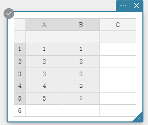
4-4. Performing 1-variable Statistical Calculations
As an example, we will use the data values below.
| Data | Frequency |
| $1$ | $1$ |
| $2$ | $2$ |
| $3$ | $3$ |
| $4$ | $2$ |
| $5$ | $1$ |
1. Input data values into column A and frequencies into column B.
2. Drag from cell A1 to cell B5 to select the range of cells between them.
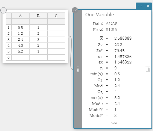
3. On the soft keyboard, click [Calculation] - [One-Variable].
• This displays one-variable statistical calculation results.
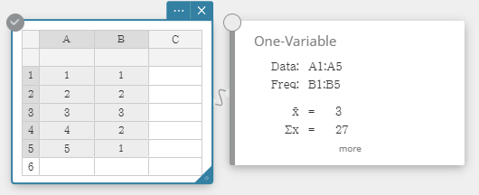
4. To display other hidden calculation result items, click [more] on the Statistical Calculation Sticky Note.
• To return the Statistical Calculation Sticky Note to its reduced size configuration, click [hide].
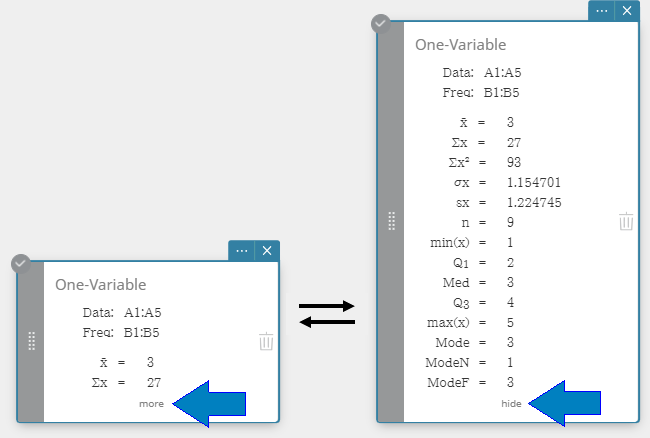
• Performing a one-variable statistical calculation displays the results below.
| ${\rm x̅}$ | sample mean |
| $\Sigma {\rm x}$ | sum of data |
| $\Sigma {\rm x}^2$ | sum of squares |
| $\sigma {\rm x}$ | population standard deviation |
| ${\rm sx}$ | sample standard deviation |
| ${\rm n}$ | sample size |
| ${\rm min(x)}$ | minimum |
| ${\rm Q}_1$ | first quartile |
| ${\rm Med}$ | median |
| ${\rm Q}_3$ | third quartile |
| ${\rm max(x)}$ | maximum |
| ${\rm Mode}$ | mode |
| ${\rm ModeN}$ | number of data mode items |
| ${\rm ModeF}$ | data mode frequency |
| When ${\rm Mode}$ has multiple solutions, they are all displayed. | |
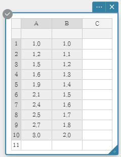
4-5. Drawing a Regression Graph
In this example, we will use the data values below to draw a scatter plot, linear regression graph, and a quadratic regression graph.
|
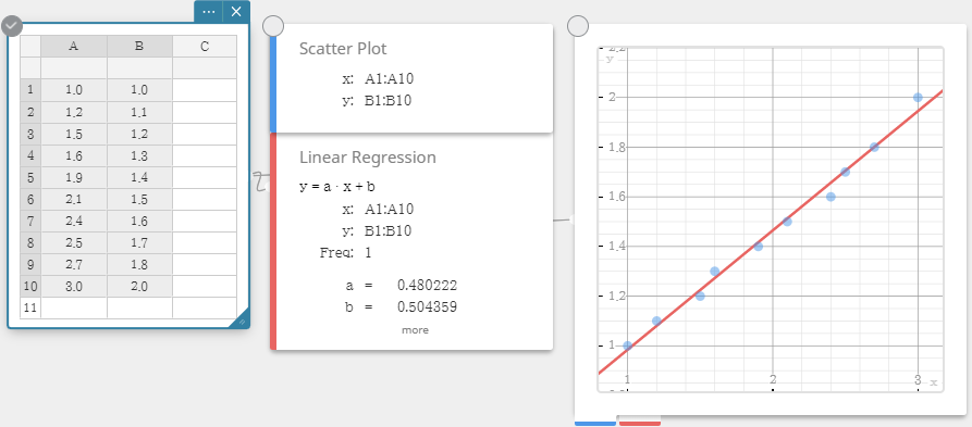
1. Input data values into columns A and B.
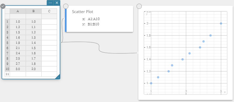
2. Drag from cell A1 to cell B10 to select the range of cells between them.
3. On the soft keyboard, click [Graph] - [Scatter Plot].
• This creates a Scatter Plot Sticky Note and draws a scatter plot on the Graph Sticky Note simultaneously.
4. On the soft keyboard, click .

5. On the soft keyboard, click [Regression] - [Linear Regression].
• This creates a Linear Regression Sticky Note and draws a linear regression graph on the Graph Sticky Note simultaneously.
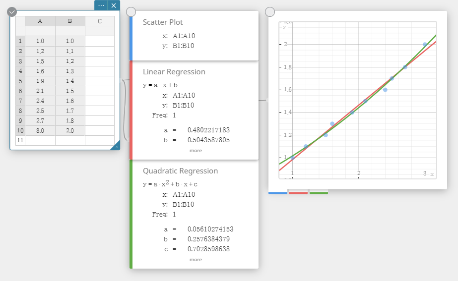
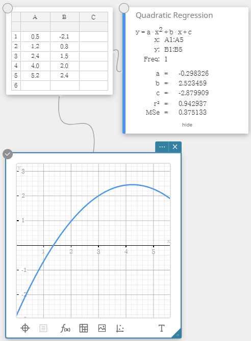
6. On the soft keyboard, click [Quadratic Regression].
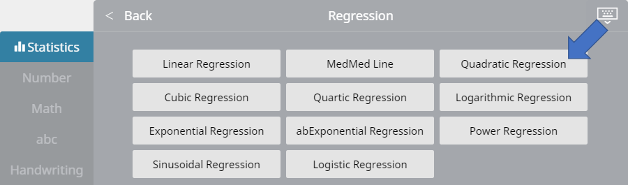
• This creates a Quadratic Regression Sticky Note and draws a quadratic regression graph on the Graph Sticky Note simultaneously.
4-6. Drawing a Histogram
As an example, we will use the data values below.
| Data | Frequency |
| $1$ | $1$ |
| $2$ | $2$ |
| $3$ | $3$ |
| $4$ | $2$ |
| $5$ | $1$ |
1. Input data values into column A and frequencies into column B.
2. Drag from cell A1 to cell B5 to select the range of cells between them.
3. On the soft keyboard, click [Graph] - [Histogram].
• This creates a Histogram Sticky Note and draws a histogram on the Graph Sticky Note simultaneously.
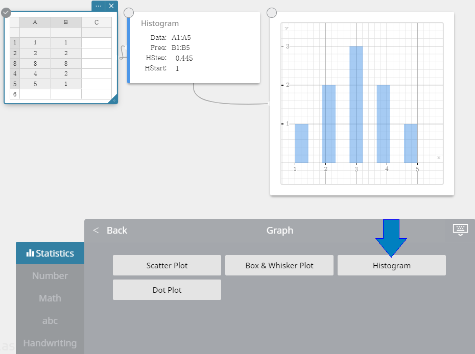
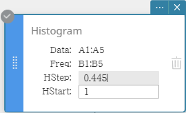
Note
- You can change the histogram draw start value (HStart) and step value (HStep), if you want. On the Histogram Sticky Note, click HStart or HStep and then input the value you want.
4-7. Drawing a Box-and-whisker Diagram
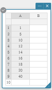
As an example, we will use the data values below.
| Data |
| $1$ |
| $5$ |
| $10$ |
| $12$ |
| $14$ |
| $16$ |
| $18$ |
| $20$ |
| $40$ |
1. Input data values into column A.
2. Drag from cell A1 to cell A9 to select the range of cells between them.
3. On the soft keyboard, click [Graph] - [Box & Whisker Plot].
• This creates a Box & Whisker Plot Sticky Note and draws s box-and-whisker diagram on the Graph Sticky Note simultaneously.
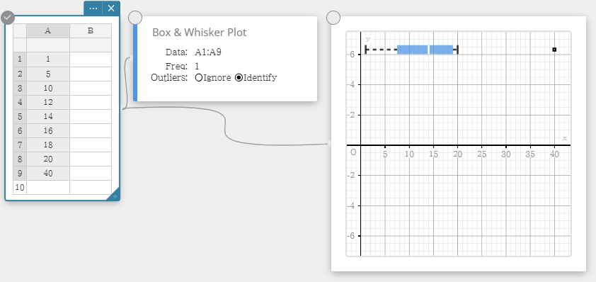
Note
- You can display outlier values, if you want. To do so, select [Identify] for the Outliers item of the Box & Whisker Plot Sticky Note.

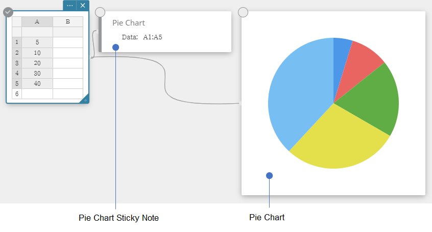
4-8. Drawing a Circle Graph
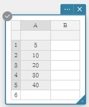
As an example, we will use the data values below.
| Data |
| $5$ |
| $10$ |
| $20$ |
| $30$ |
| $40$ |
1. Input data values into column A.
2. Drag from cell A1 to cell A5 to select the range of cells between them.
3. On the soft keyboard, click [Graph] - [Pie Chart].
• This creates a Pie Chart Sticky Note and draws a pie graph on a separate Sticky Note simultaneously.
4-9. Scatter Plot Operations
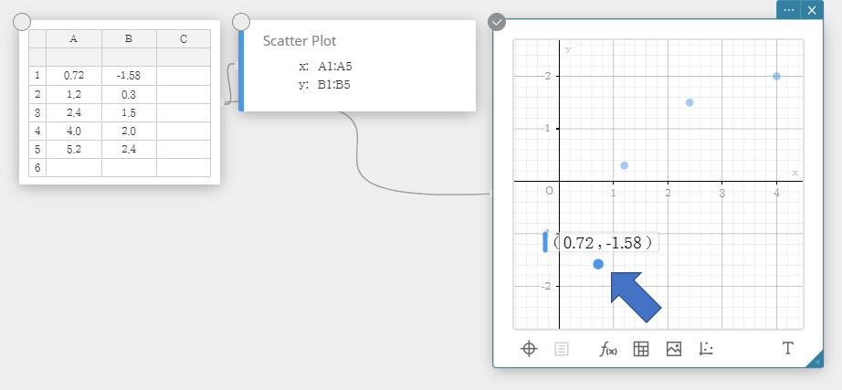
4-9-1. To move the points of a scatter plot
As an example, we will use the data values below.
| Data | Frequency |
| $0.5$ | $-2.1$ |
| $1.2$ | $0.3$ |
| $2.4$ | $1.5$ |
| $4.0$ | $2.0$ |
| $5.2$ | $2.4$ |
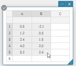
1. Input data values into columns A and B.
2. Drag from cell A1 to cell B5 to select the range of cells between them.
3. On the soft keyboard, click [Graph] - [Scatter Plot].
• This creates a Scatter Plot Sticky Note and Graph Sticky Note, and draws a scatter plot on the Graph Sticky Note.
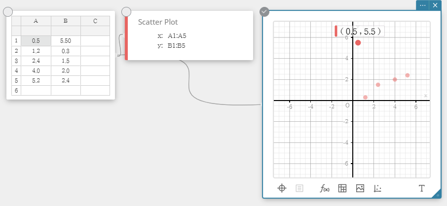
4. To move a scatter plot point, drag it.
• This will also change the Statistical Data Sticky Note values to the coordinates of the destination.
4-9-2. To lock a cell
Note
- When a cell is locked, its data value will not change even if you try to move its scatter plot point. For example, if you lock a column A cell, the corresponding scatter plot point cannot be moved along the x-axis.
1. Continuing from the procedure under "4-9-1. To move the points of a scatter plot", select cell A1.
2. Click the Statistical Data Sticky Note Settings button ( ).
).
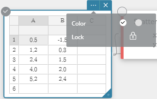
3. Click the lock icon ( ) next to [Lock].
・This locks cell A1. If you drag the scatter plot point that corresponds to cells A1 and B1, movement will not be possible along the x-axis.
4-9-3. To unlock a cell
1. Select the locked cell that you want to unlock.
2. Click the Statistical Data Sticky Note Settings button ( ).
).

3. Click the unlock icon ( ) next to [UnLock].
4-10. Performing a One-Sample Z-Test
4-10 -1. To specify the number of data samples and then perform a one-sample Z-test
Example:
- Sample size: ($n$) = 48
- Sample mean: ($\overline{x}$) = 24.5
- Null hypothesis: $\mu \ne 0$
- Standard deviation: $\sigma = 3$
1. Create a Statistical Data Sticky Note.
2. On the soft keyboard, click [Test] - [One-Sample Z-Test].
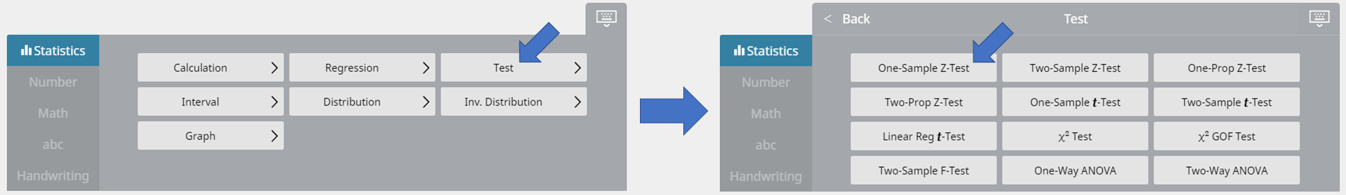
• This creates a One-Sample Z-Test Sticky Note.
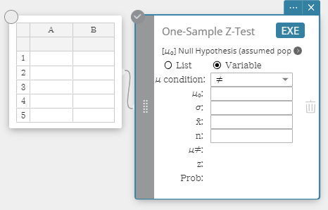
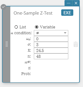
3. Configure settings as shown below.
- $\mu$ condition: On the menu that appears, select "$\ne$" .
- $\mu_0$ : Input $0$ .
- $\sigma$: Input $3$ .
- $\overline{x}$ : Input $24.5$ .
- $n$ : Input $48$ .
4. Click [EXE].
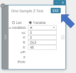
• This displays the calculation results and the graph.
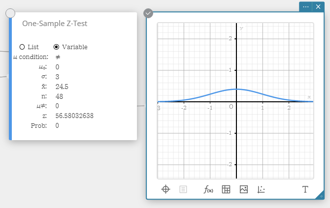
- $ \mu \ne $ ... population mean value condition
- $ z $ ... zvalue
- Prob ... pvalue
- $ \overline{x} $ ... sample mean
- $ n $ ... sample size
4-10-2. To use lists to perform a one-sample Z-test
1. Input the following list names: List 1 for column A, List 2 for column B.
2. Input the data value in the table below.
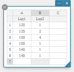
3. Drag from cell A1 to cell B6 to select the range of cells.
4. On the soft keyboard, click [Test] - [One-Sample Z-Test].
• This creates a One-Sample Z-Test Sticky Note.
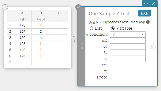
5. Click "List".
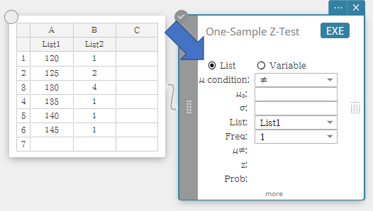
6. Configure settings as shown below.
- $\mu$ condition: On the pulldown menu that appears, select "$\gt$".
- $\mu_0$ : Input $120$ .
- $\sigma$: Input $19$ .
-
List: On the menu that appears, select "List1".
Freq: On the menu that appears, select "List2".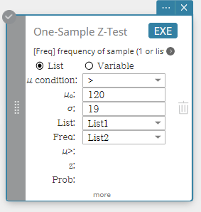
7. Click [EXE].
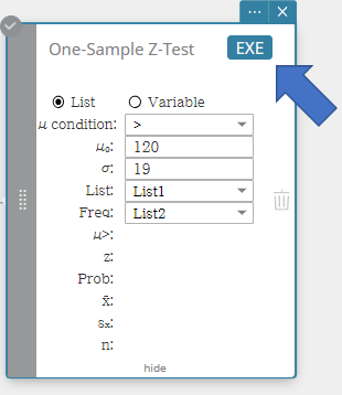
• This displays the calculation results and the graph.
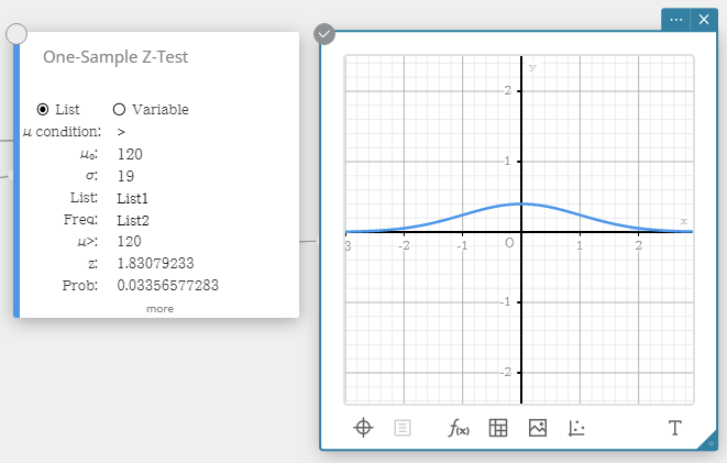
- $ \mu > $ ... population mean value condition
- $ z $ ... zvalue
- Prob ... pvalue
- $ \overline{x} $ ... sample mean
- $ s_x $ ... sample standard deviation
- $ n $ ... sample size
4-11. Statistical Calculations and Graphs
4-11-1. Statistical Calculations
| One-Variable | |
|---|---|
|
This displays the calculation results of single-variable statistics. $x ̅$ ... sample mean $\Sigma x$ ... sum of data $\Sigma x^2$ ... sum of squares $\sigma x$ ... population standard deviation $sx$ ... sample standard deviation $n$ ... sample size $minX$ ... minimum $Q1$ ... first quartile $Med$ .... median $Q3$ ... third quartile $maxX$ ... maximum $Mode$ ... mode $ModeN$ ... number of data mode items $ModeF$ ... data mode frequency When $Mode$ has multiple solutions, they are all displayed. |
 |
| Two-Variable | |
|
This displays the calculation results of paired-variable statistics. $x ̅$ ... sample mean $\Sigma x$ ... sum of data $\Sigma x^2$ ... sum of squares $\sigma x$ ... population standard deviation $sx$ ... sample standard deviation $n$ ... sample size $y ̅$ ... sample mean $\Sigma y$ ... sum of data $\Sigma y^2$ ............. sum of squares $\sigma y$ ... population standard deviation $sy$ ... sample standard deviation $\Sigma xy$ ... sum of the products XList and YList data $minX$ ... minimum $maxX$ ... maximum $minY$... minimum $maxY$ ... maximum |
 |
4-11-2. Regression Calculations and Graphs
| Linear Regression | |
|---|---|
|
Linear regression uses the method of least squares to determine the equation that best fits your data points, and returns values for the slope and y-intercept. The graphic representation of this relationship is a linear regression graph. $y = a \cdot x + b$ $a$ ... regression coefficient (slope) $b$ ... regression constant term (y-intercept) $r$ .... correlation coefficient $r^2$ ... coefficient of determination $MSe$ ... mean square error |
 |
| MedMed Regression | |
|
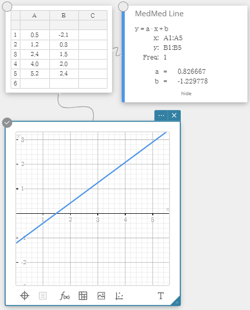
When you suspect that the data contains extreme values, you should use the Med-Med graph (which is based on medians) in place of the linear regression graph. Med-Med graph is similar to the linear regression graph, but it also minimizes the effects of extreme values. $y = a \cdot x + b$ $a$ ... regression coefficient (slope) $b$ ... regression constant term (y-intercept) |
 |
| Quadratic Regression | |
|
Quadratic regression graph uses the method of least squares to draw a curve that passes the vicinity of as many data points as possible. This graph can be expressed as quadratic regression expression. $y = a \cdot x^2 + b \cdot x + c$ $a$ ... regression second coefficient $b$ ... regression first coefficient $c$ ... regression constant term (y-intercept) $r^2$ ... coefficient of determination $MSe$ ... mean square error |
 |
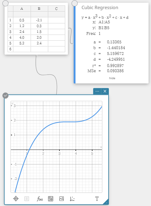
| Cubic Regression | |
|
Cubic regression graph uses the method of least squares to draw a curve that passes the vicinity of as many data points as possible. This graph can be expressed as cubic regression expression. $y = a \cdot x^3 + b \cdot x^2 + c \cdot x + d$ $a$ ... regression third coefficient $b$ ... regression second coefficient $c$ ... regression first coefficient $d$ ... regression constant term (y-intercept) $r^2$ ... coefficient of determination $MSe$ ... mean square error |
 |
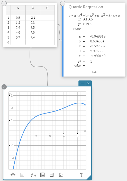
| Quartic Regression | |
|
Quartic regression graph uses the method of least squares to draw a curve that passes the vicinity of as many data points as possible. This graph can be expressed as quartic regression expression. $y = a \cdot x^4 + b \cdot x^3 + c \cdot x^2 + d \cdot x + e$ $a$ ... regression fourth coefficient $b$ ... regression third coefficient $c$ ... regression second coefficient $d$ ... regression first coefficient $e$ ... regression constant term (y-intercept) $r^2$ ... coefficient of determination $MSe$ ... mean square error |
 |
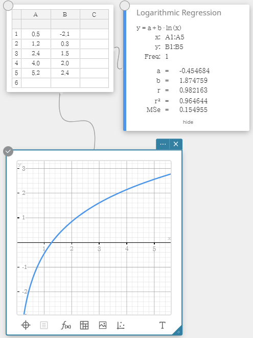
| Logarithmic Regression | |
|
Logarithmic regression expresses $y$ as a logarithmic function of $x$. The normal logarithmic regression formula is $y=a+b \cdot \ln(x)$. If we say that $X=\ln(x)$, then this formula corresponds to the linear regression formula $y=a+b \cdot X$. $y = a + b \cdot \ln(x)$ $a$ ... regression constant term $b$ ... regression coefficient $r$ .... correlation coefficient $r^2$ ... coefficient of determination $MSe$ ... mean square error |
 |
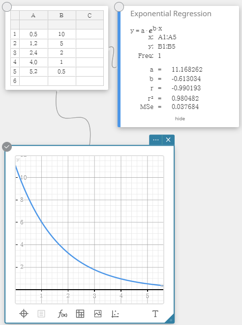
| Exponential Regression | |
|
Exponential regression can be used when $y$ is proportional to the exponential function of $x$. The normal exponential regression formula is $y=a \cdot e^{b \cdot x}$. If we obtain the logarithms of both sides, we get $\ln(y)=\ln(a)+b \cdot x$. Next, if we say that $Y=\ln(y)$ and $A=\ln(a)$, the formula corresponds to the linear regression formula $Y=A+b \cdot x$. $y = a \cdot e^{b \cdot x}$ $a$ ... regression coefficient $b$ ... regression constant term $r$ .... correlation coefficient $r^2$ ... coefficient of determination $MSe$ ... mean square error |
 |
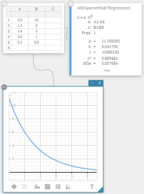
| abExponential Regression | |
|
Exponential regression can be used when $y$ is proportional to the exponential function of $x$. The normal exponential regression formula in this case is $y=a \cdot b^x$. If we take the natural logarithms of both sides, we get $\ln(y)=\ln(a)+(\ln(b)) \cdot x$. Next, if we say that $Y=\ln(y)$, $A=\ln(a)$ and $B=\ln(b)$, the formula corresponds to the linear regression formula $Y=A+B \cdot x$. $y = a \cdot b^x$ $a$ ... regression constant term $b$ ... regression coefficient $r$ .... correlation coefficient $r^2$ ... coefficient of determination $MSe$ ... mean square error |
 |
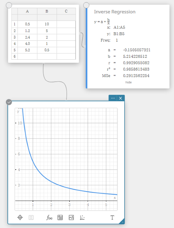
| Inverse Regression | |
|
Inverse regression expresses $y$ as an inverse function of $x$. The normal inverse regression formula is $y=a+b/x$. If we say that $X=1/x$, then this formula corresponds to the linear regression formula $y=a+b \cdot X$. $y = a + b / x$ $a$ ... regression constant term $b$ ... regression coefficient $r$ .... correlation coefficient $r^2$ ... coefficient of determination $MSe$ ... mean square error |
 |
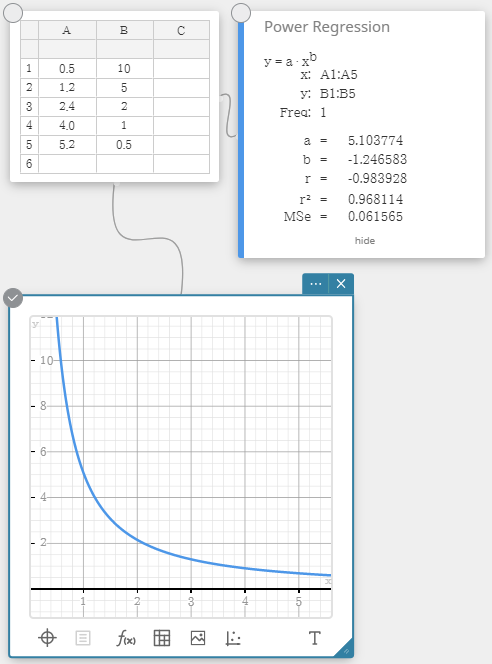
| Power Regression | |
|
Power regression can be used when $y$ is proportional to the power of $x$. The normal power regression formula is $y=a \cdot x^b$. If we obtain the natural logarithms of both sides, we get $\ln(y)=\ln(a)+b \cdot \ln(x)$. Next, if we say that $X=\ln(x)$, $Y=\ln(y)$, and $A=\ln(a)$, the formula corresponds to the linear regression formula $Y=A+b \cdot X$. $y = a \cdot x^b$ $a$ ... regression coefficient $b$ ... regression power $r$ .... correlation coefficient $r^2$ ... coefficient of determination $MSe$ ... mean square error |
 |
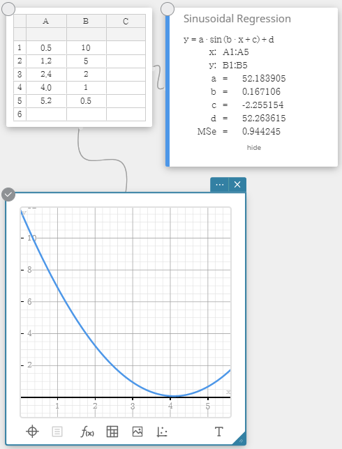
| Sinusoidal Regression | |
|
Sinusoidal regression is best for data that repeats at a regular fixed interval over time. $y = a \cdot \sin( b \cdot x + c ) + d$ $a$, $b$, $c$, $d$ ... regression coefficient $MSe$ ... mean square error |
 |
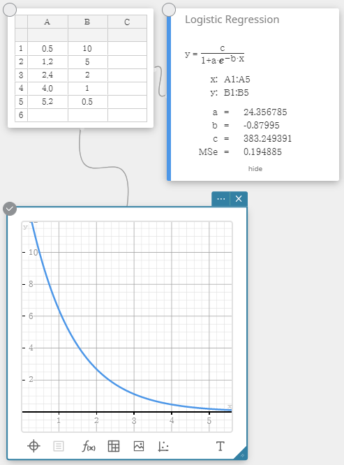
| Logistic Regression | |
|
Logistic regression is best for data whose values continually increase over time, until a saturation point is reached. $y=\cfrac{c}{1+a \cdot e^{-b \cdot x}}$ $a$, $b$, $c$ ... regression coefficient $MSe$ ... mean square error |
 |
4-11-3. Tests
| One-Sample Z-Test | |
|---|---|
|
Tests a single sample mean against the known mean of the null hypothesis when the population standard deviation is known. The normal distribution is used for the One-Sample Z-Test. $Z=\cfrac{\overline{x}-\mu_{0}}{\cfrac{\sigma}{\sqrt{n}}}$ $\overline{x}$ : sample mean $\mu_{0}$ : assumed population mean $\sigma$ : population standard deviation $n$ : sample size |
 |
|
Data type: Variable ・Input Terms
・Output Terms
Data type: List ・Input Terms
・Output Terms
|
|
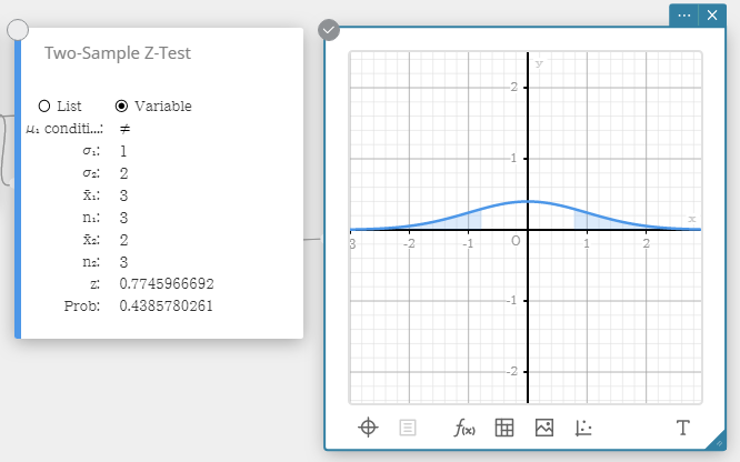
| Two-Sample Z-Test | |
|
Tests the difference between two means when the standard deviations of the two populations are known.
The normal distribution is used for the Two-Sample Z-Test. $ Z=\cfrac{ \overline{x}_{1} - \overline{x}_{2} }{ \sqrt{ \cfrac{{\sigma_{1}}^2}{n_{1}} + \cfrac{{\sigma_{2}}^2}{n_{2}} } } $ $ \overline{x}_{1} $ : sample mean of sample 1 data $ \overline{x}_{2} $ : sample mean of sample 2 data $ \sigma_{1} $ : population standard deviation of sample 1 $ \sigma_{2} $ : population standard deviation of sample 2 $ n_{1} $ : size of sample 1 $ n_{2} $ : size of sample 2 |
 |
|
Data type: Variable ・Input Terms
・Output Terms
Data type: List ・Input Terms
・Output Terms
|
|
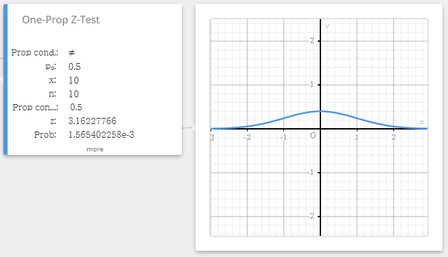
| One-Prop Z-Test (One-Proportion Z-Test) | |
|
Tests a single sample proportion against the known proportion of the null hypothesis.
The normal distribution is used for the One-Proportion Z-Test. $Z = \cfrac{ \cfrac{x}{n} - p_{0} }{ \sqrt{ \cfrac{ p_{0}(1-p_{0}) }{n} }}$ $p_{0}$ : expected sample proportion $n$ : sample size |
 |
|
・Input Terms
・Output Terms
|
|
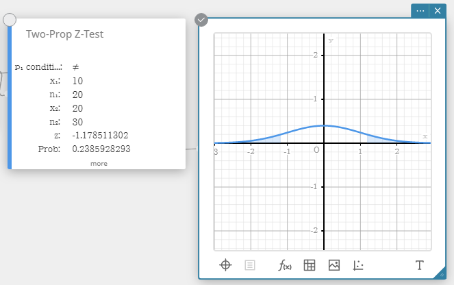
| Two-Prop Z-Test (Two-Proportion Z-Test) | |
|
Tests the difference between two sample proportions. The normal distribution is used for the Two-Proportion Z-Test. $ Z = \cfrac{ \cfrac{x_{1}}{n_{1}} - \cfrac{x_{2}}{n_{2}} }{ \sqrt{ \hat{p} \left(1-\hat{p} \right) \left( \cfrac{1}{n_{1}} + \cfrac{1}{n_{2}} \right) } }$ $x_{1}$ : data value of sample 1 $x_{2}$ : data value of sample 2 $n_{1}$ : size of sample 1 $n_{2}$ : size of sample 2 $\hat{p}$ : estimated sample proportion |
 |
|
・Input Terms
・Output Terms
|
|
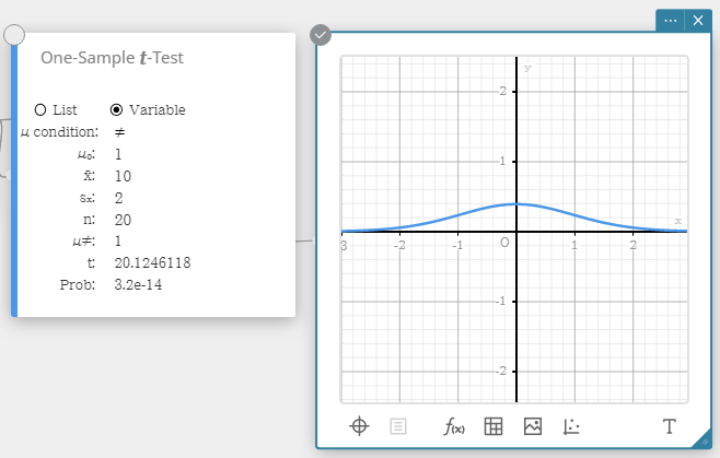
| One-Sample t-Test | |
|
Tests a single sample mean against the known mean of the null hypothesis when the population standard deviation is unknown.
The t distribution is used for the One-Sample t-Test. $t = \cfrac{ \overline{x} - \mu_{0} }{ \cfrac{ s_{x} }{ \sqrt{n} } }$ $\overline{x}$ : sample mean $\mu_{0}$ : assumed population mean $s_{x}$ : sample standard deviation $n$ : sample size |
 |
|
Data type: Variable ・Input Terms
・Output Terms
Data type: List ・Input Terms
・Output Terms
|
|
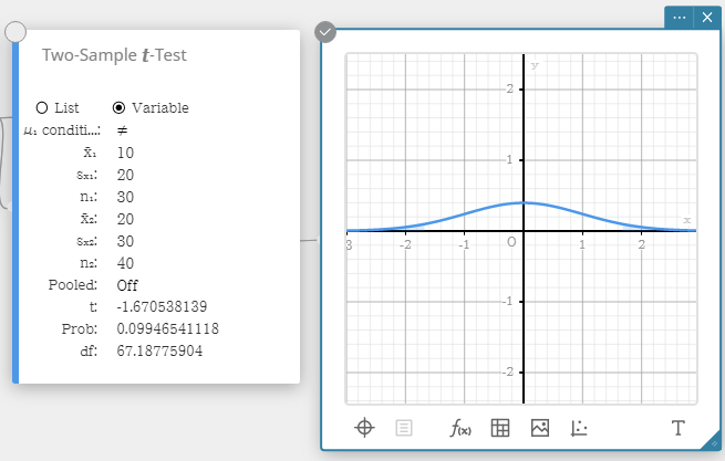
| Two-Sample t-Test | |
|
Tests the difference between two means when the standard deviations of the two populations are unknown. The t distribution is used for the Two-Sample t-Test. ・When the two population standard deviations are equal (pooled) $t=(\overline{x}_{1}-\overline{x}_{2})/\sqrt{{s_{p}}^2(1/n_1+1/n_2)}$ $df=n_1+n_2-2$ $s_p=\sqrt{ ( (n_1-1){s_{x_1}}^2 + (n_2-1){s_{x_2}}^2 ) / (n_1+n_2-2) }$ ・When the two population standard deviations are not equal (not pooled) $t=(\overline{x}_{1}-\overline{x}_{2})/\sqrt{ {s_{x_1}}^2/n_1 + {s_{x_2}}^2/n_2 }$ $df = 1 / ( C^2/(n_1-1) + (1-C)^2/(n_2-1) )$ $C = ({s_{x_1}}^2/n_1)/({s_{x_1}}^2/n_1+{s_{x_2}}^2/n_2)$ $x_1$: sample mean of sample 1 data $x_2$: sample mean of sample 2 data $s_{x_1}$ : sample standard deviation of sample 1 $s_{x_2}$ : sample standard deviation of sample 2 $s_p$ : pooled sample standard deviation $n_1$ : size of sample 1 $n_2$ : size of sample 2 |
 |
|
Data type: Variable ・Input Terms
・Output Terms
Data type: List ・Input Terms
・Output Terms
|
|
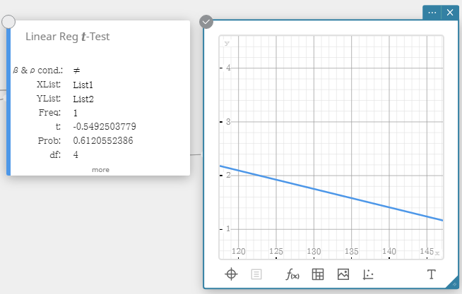
| Linear Reg t-Test (Linear Regression t-Test) | |
|
Tests the linear relationship between the paired variables (x, y). The method of least squares is used to determine a and b, which are the coefficients of the regression formula $y = a + b \cdot x$.
The p-value is the probability of the sample regression slope (b) provided that the null hypothesis is true, $\beta=0$. The t distribution is used for the Linear Regression t-Test. $t=r\sqrt{\cfrac{n-2}{1-r^2}}$ $b=\sum_{i=1}^{n}(x_i-\overline{x})(y_i-\overline{y})/\sum_{i=1}^{n}(x_i-\overline{x})^2$ $a=\overline{y}-b\overline{x}$ $a$ : regression constant term (y-intercept) $b$ : regression coefficient (slope) $n$ : sample size (n ≥ 3) $r$ : correlation coefficient $r^2$ : coefficient of determination |
 |
|
・Input Terms
・Output Terms
|
|
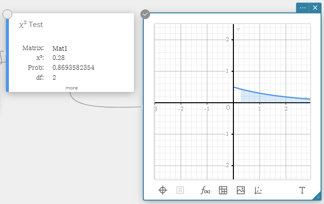
| χ2 Test | |
|
Tests the independence of two categorical variables arranged in matrix form. The χ2 test for independence compares the observed matrix to the expected theoretical matrix. The χ2 distribution is used for the χ2 test. ・The minimum size of the matrix is 1×2. An error occurs if the matrix has only one column. ・The result of the expected frequency calculation is stored in the system variable named “Expected”. $$ \chi^2 = \sum_{i=1}^{k}\sum_{j=1}^{l} \cfrac{(x_{ij}-F_{ij})^2}{F_{ij}} $$ $$ F_{ij}=\cfrac{ \sum_{i=1}^{k}x_{ij} \times \sum_{j=1}^{l}x_{ij} }{ \sum_{i=1}^{k} \sum_{j=1}^{l}x_{ij} } $$ $ x_{ij}$ : The element at row i, column j of the observed matrix $ F_{ij}$ : The element at row i, column j of the expected matrix |
 |
|
・Input Terms
・Output Terms
|
|
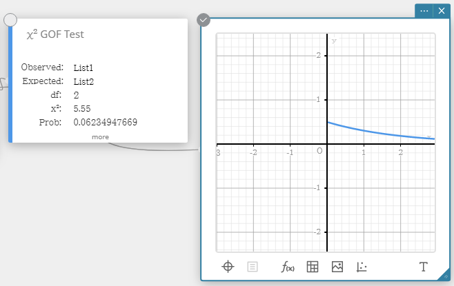
| χ2 GOF Test (χ2 Goodness-Of-Fit Test) | |
|
Tests whether the observed count of sample data fits a certain distribution. For example, it can be used to determine conformance with normal distribution or binomial distribution. $\chi^2=\sum_{i}^{k} \cfrac{ (O_i - E_i )^2 }{E_i}$ $$Contrib = \left\{ \cfrac{ (O_1 - E_1 )^2 }{E_1} \ \cfrac{ (O_2 - E_2 )^2 }{E_2} \cdots \cfrac{ (O_k - E_k )^2 }{E_k} \right\} $$ $O_i$ : The i-th element of the observed list $E_i$ : The i-th element of the expected list |
 |
|
・Input Terms
・Output Terms
|
|
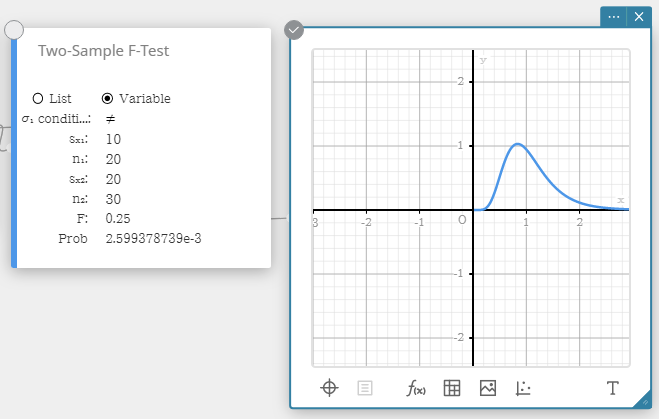
| Two-Sample F-Test | |
|
Tests the ratio between sample variances of two independent random samples. The F distribution is used for the Two-Sample F-Test. $F=\cfrac{{S_{x_1}}^2}{{S_{x_2}}^2}$ |
 |
|
Data type: Variable ・Input Terms
・Output Terms
Data type: List ・Input Terms
・Output Terms
|
|
| One-Way ANOVA (One-Way analysis of variance) | |
| Tests the hypothesis that the population means of multiple populations are equal. It compares the mean of one or more groups based on one independent variable or factor. | 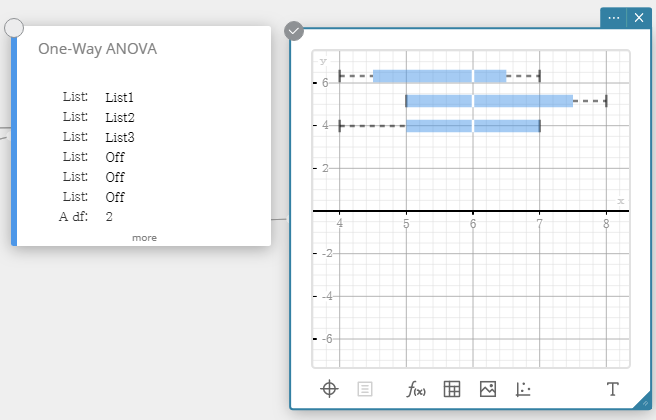 |
|
・Input Terms
・Output Terms
|
|
| Two-Way ANOVA (Two-Way analysis of variance) | |
| Tests the hypothesis that the population means of multiple populations are equal. It examines the effect of each variable independently as well as their interaction with each other based on a dependent variable. | 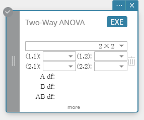 |
|
・Input Terms
・Output Terms
|
|
4-11-4. Confidence Intervals
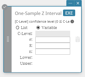
| One-Sample Z Interval | |
|---|---|
|
Calculates the confidence interval for the population mean based on a sample mean and known population standard deviation. $Lower = \overline{x}-Z \left(\cfrac{\alpha}{2} \right) \cfrac{\sigma}{\sqrt{n}}$ $Upper = \overline{x}+Z \left(\cfrac{\alpha}{2} \right) \cfrac{\sigma}{\sqrt{n}}$ α is the significance level, and 100 (1 – α)% is the confidence level. When the confidence level is 95%, for example, you would input 0.95, which produces α = 1 – 0.95 = 0.05. |
 |
|
Data type: Variable ・Input Terms
・Output Terms
Data type: List ・Input Terms
・Output Terms
|
|
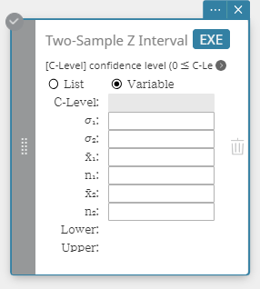
| Two-Sample Z Interval | |
|
Calculates the confidence interval for the difference between population means based on the difference between sample means when the population standard deviations are known. $Lower = \left( \overline{x}_1-\overline{x}_2 \right) -Z \left( \cfrac{\alpha}{2} \right) \sqrt{ \cfrac{{\sigma_1}^2}{n_1} + \cfrac{{\sigma_2}^2}{n_2} }$ $Upper = \left( \overline{x}_1-\overline{x}_2 \right) +Z \left( \cfrac{\alpha}{2} \right) \sqrt{ \cfrac{{\sigma_1}^2}{n_1} + \cfrac{{\sigma_2}^2}{n_2} }$ |
 |
|
Data type: Variable ・Input Terms
・Output Terms
Data type: List ・Input Terms
・Output Terms
|
|
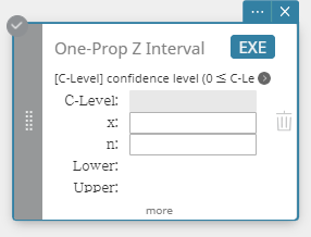
| One-Prop Z Interval (One-Proportion Z Interval) | |
|
Calculates the confidence interval for the population proportion based on a single sample proportion. $Lower = \cfrac{x}{n}-Z \left( \cfrac{\alpha}{2} \right) \sqrt{\cfrac{1}{n} \left( \cfrac{x}{n} \left( 1-\cfrac{x}{n} \right) \right) }$ $Upper = \cfrac{x}{n}+Z \left( \cfrac{\alpha}{2} \right) \sqrt{\cfrac{1}{n} \left( \cfrac{x}{n} \left( 1-\cfrac{x}{n} \right) \right) }$ |
 |
|
・Input Terms
・Output Terms
|
|
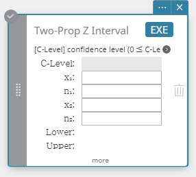
| Two-Prop Z Interval (Two-Proportion Z Interval) | |
|
Calculates the confidence interval for the difference between population proportions based on the difference between Two-Proportion Z Interval. $ Lower = \cfrac{x_1}{n_1}-\cfrac{x_2}{n_2}-Z \left( \cfrac{\alpha}{2} \right) \sqrt{ \cfrac{ \cfrac{x_1}{n_1} \left( 1-\cfrac{x_1}{n_1} \right) }{n_1} + \cfrac{ \cfrac{x_2}{n_2} \left( 1-\cfrac{x_2}{n_2} \right) }{n_2} } $ $ Upper = \cfrac{x_1}{n_1}-\cfrac{x_2}{n_2}+Z \left( \cfrac{\alpha}{2} \right) \sqrt{ \cfrac{ \cfrac{x_1}{n_1} \left( 1-\cfrac{x_1}{n_1} \right) }{n_1} + \cfrac{ \cfrac{x_2}{n_2} \left( 1-\cfrac{x_2}{n_2} \right) }{n_2} } $ |
 |
|
・Input Terms
・Output Terms
|
|
| One-Sample t Interval | |
|
Calculates the confidence interval for the population mean based on a sample mean and a sample standard deviation when the population standard deviation is not known. $Lower = \overline{x}-t_{n-1} \left( \cfrac{\alpha}{2} \right) \cfrac{s_x}{\sqrt{n}}$ $Upper = \overline{x}+t_{n-1} \left( \cfrac{\alpha}{2} \right) \cfrac{s_x}{\sqrt{n}}$ |
 |
|
Data type: Variable ・Input Terms
・Output Terms
Data type: List ・Input Terms
・Output Terms
|
|
| Two-Sample t Interval | |
|
Calculates the confidence interval for the difference between population means based on the difference between sample means and sample standard deviations when the population standard deviations are not known. When the two population standard deviations are equal (pooled) $$Lower = \left( \overline{x}_1-\overline{x}_2 \right) -t_{n_1+n_2-2} \left( \cfrac{\alpha}{2} \right) \sqrt{{s_p}^2 \left( \cfrac{1}{n_1}+\cfrac{1}{n_2} \right) }$$ $$Upper = \left( \overline{x}_1-\overline{x}_2 \right) +t_{n_1+n_2-2} \left( \cfrac{\alpha}{2} \right) \sqrt{{s_p}^2 \left( \cfrac{1}{n_1}+\cfrac{1}{n_2} \right) }$$ When the two population standard deviations are not equal (not pooled) $$Lower = \left( \overline{x}_1-\overline{x}_2 \right) -t_{df} \left( \cfrac{\alpha}{2} \right) \sqrt{ \left( \cfrac{{S_{x_1}}^2}{n_1}+\cfrac{{S_{x_2}}^2}{n_2} \right) }$$ $$Upper = \left( \overline{x}_1-\overline{x}_2 \right) +t_{df} \left( \cfrac{\alpha}{2} \right) \sqrt{ \left( \cfrac{{S_{x_1}}^2}{n_1}+\cfrac{{S_{x_2}}^2}{n_2} \right) }$$ $$df = \cfrac{1}{\cfrac{C^2}{n_1-1} + \cfrac{ \left( 1-C \right) ^2}{n_2-1}}$$ $$C=\cfrac{\cfrac{{S_{x_1}}^2}{n_1}}{ \left( \cfrac{{S_{x_1}}^2}{n_1} + \cfrac{{S_{x_2}}^2}{n_2} \right) }$$ |
 |
|
Data type: Variable ・Input Terms
・Output Terms
Data type: List ・Input Terms
・Output Terms
|
|
4-11-5. Distribution
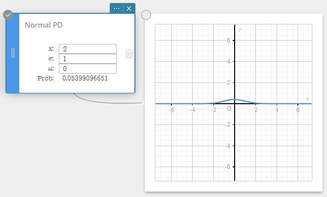
| Normal PD (Normal Probability Density) | |
|---|---|
|
Calculates the normal probability density for a specified value. Specifying σ = 1 and μ= 0 produces standard normal distribution. $$f(x)=\cfrac{1}{\sqrt{2\pi}\sigma}e^{-\cfrac{(x-\mu)^2}{2\sigma^2}} \qquad (\sigma>0)$$ |
 |
|
・Input Terms
・Output Terms
|
|
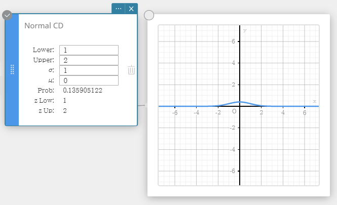
| Normal CD (Normal Cumulative Distribution) | |
|
Calculates the cumulative probability of a normal distribution between a lower bound (a) and an upper bound (b). $$p=\frac{1}{\sqrt{2\pi}\sigma}\int_a^b e^{ \scriptscriptstyle -\frac{(x-\mu)^2}{2\sigma^2} }dx$$ |
 |
|
・Input Terms
・Output Terms
|
|
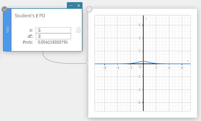
| Student’s t PD (Student’s t Probability Density) | |
|
Calculates the Student’s t probability density for a specified value. $$f(x) =\cfrac{\Gamma \left( \cfrac{df+1}{2} \right) }{\Gamma \left( \cfrac{df}{2} \right) }\cfrac{ \left( 1+\cfrac{x^2}{df} \right) ^{-\cfrac{df+1}{2}}}{\sqrt{\pi \cdot df}}$$ |
 |
|
・Input Terms
・Output Terms
|
|
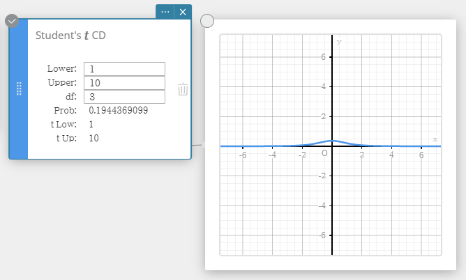
| Student’s t CD (Student’s t Cumulative Distribution) | |
|
Calculates the cumulative probability of a Student’s t distribution between a lower bound (a) and an upper bound (b). $$ p=\cfrac{\Gamma \left( \cfrac{df+1}{2} \right) }{\Gamma \left( \cfrac{df}{2} \right) \sqrt{\pi \cdot df}}\int_a^b \left( 1+\cfrac{x^2}{df} \right) ^{-\cfrac{df+1}{2}}dx $$ |
 |
|
・Input Terms
・Output Terms
|
|
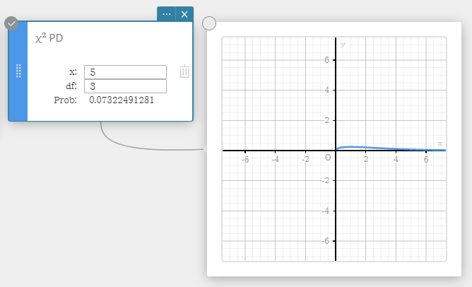
| χ2 PD (χ2 Probability Density) | |
|
Calculates the χ2 probability density for a specified value. $$f \left( x \right) =\cfrac{1}{\Gamma \left( \cfrac{df}{2} \right) } \left( \cfrac{1}{2} \right) ^{\cfrac{df}{2}}x^{\cfrac{df}{2}-1}e^{-\cfrac{x}{2}}$$ |
 |
|
・Input Terms
・Output Terms
|
|
| χ2 CD (χ2 Cumulative Distribution) | |
| Calculates the cumulative probability of a χ2 distribution between a lower bound and an upper bound. $$p=\cfrac{1}{\Gamma \left( \cfrac{df}{2} \right) } \left( \cfrac{1}{2} \right) ^{\cfrac{df}{2}}\int_a^b x^{\cfrac{df}{2}-1}e^{-\cfrac{x}{2}}dx$$ | 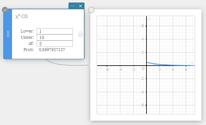 |
|
・Input Terms
・Output Terms
|
|
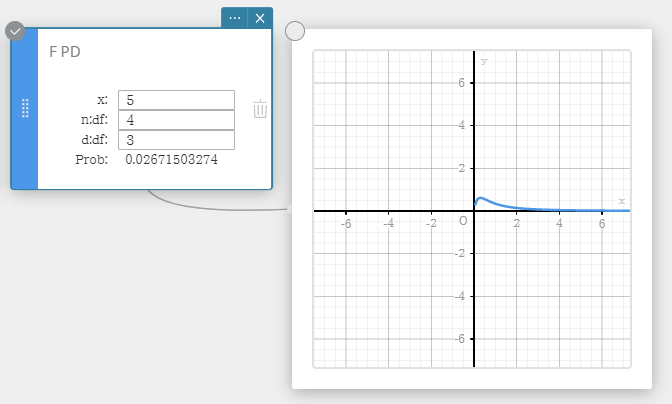
| F PD (F Probability Density) | |
|
Calculates the F probability density for a specified value. $$f(x)=\cfrac{\Gamma \left( \cfrac{n+d}{2} \right) }{\Gamma \left( \cfrac{n}{2} \right) \Gamma \left( \cfrac{d}{2} \right) } \left( \cfrac{n}{d} \right) ^{\cfrac{n}{2}}x^{\cfrac{n}{2}-1} \left( 1+\cfrac{n \cdot x}{d} \right) ^{-\cfrac{n+d}{2}}$$ |
 |
|
・Input Terms
・Output Terms
|
|
| F CD (F Cumulative Distribution) | |
| Calculates the cumulative probability of an F distribution between a lower bound and an upper bound. $$p=\cfrac{\Gamma \left( \cfrac{n+d}{2} \right) }{\Gamma \left( \cfrac{n}{2} \right) \Gamma \left( \cfrac{d}{2} \right) } \left( \cfrac{n}{d} \right) ^{\cfrac{n}{2}}\int_a^b x^{\cfrac{n}{2}-1} \left( 1+\cfrac{n \cdot x}{d} \right) ^{-\cfrac{n+d}{2}}dx$$ | 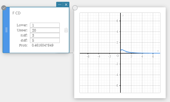 |
|
・Input Terms
・Output Terms
|
|
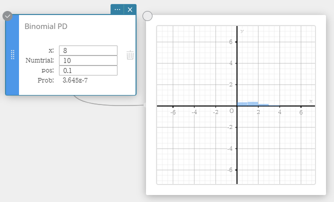
| Binomial PD (Binomial Distribution Probability) | |
|
Calculates the probability in a binomial distribution that success will occur on a specified trial. $$f(x)={}_nC_xp^x(1-p)^{n-x} \qquad (x=0,1,\cdots \cdots,n)$$ $p$ : probability of success (0 ≤ p ≤ 1) $n$ : number of trials |
 |
|
・Input Terms
・Output Terms
|
|
| Binomial CD (Binomial Cumulative Distribution) | |
| Calculates the cumulative probability in a binomial distribution that success will occur on or before a specified trial. | 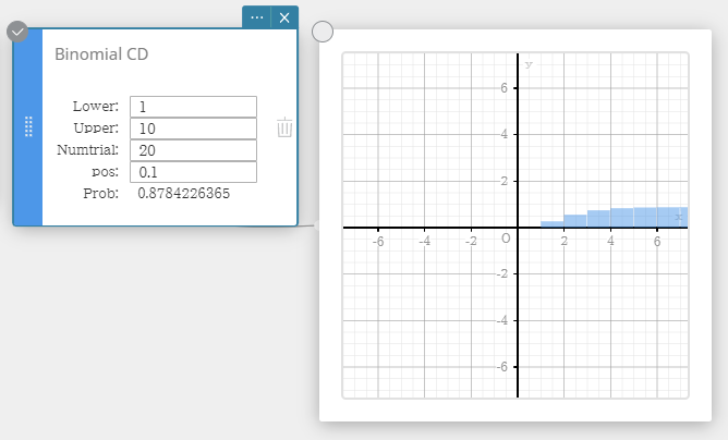 |
|
・Input Terms
・Output Terms
|
|
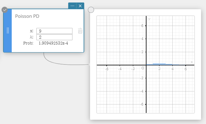
| Poisson PD (Poisson Distribution Probability) | |
|
Calculates the probability in a Poisson distribution that success will occur on a specified trial. $$f(x)=\cfrac{e^{-\lambda} \lambda^x}{x!} \qquad (x=0,1,2,\cdots)$$ |
 |
|
・Input Terms
・Output Terms
|
|
| Poisson CD (Poisson Cumulative Distribution) | |
| Calculates the cumulative probability in a Poisson distribution that success will occur on or before a specified trial. | 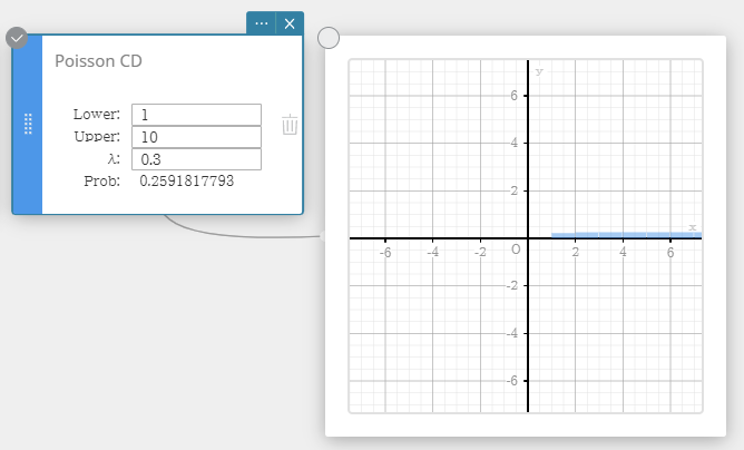 |
|
・Input Terms
・Output Terms
|
|
| Geometric PD (Geometric Distribution Probability) | |
| Calculates the probability in a geometric distribution that the success will occur on a specified trial. $$ f(x)=p(1-p)^{x-1} \qquad (x=1,2,3,\cdots) $$ | 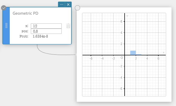 |
|
・Input Terms
・Output Terms
|
|
| Geometric CD (Geometric Cumulative Distribution) | |
| Calculates the cumulative probability in a geometric distribution that the success will occur on or before a specified trial. | 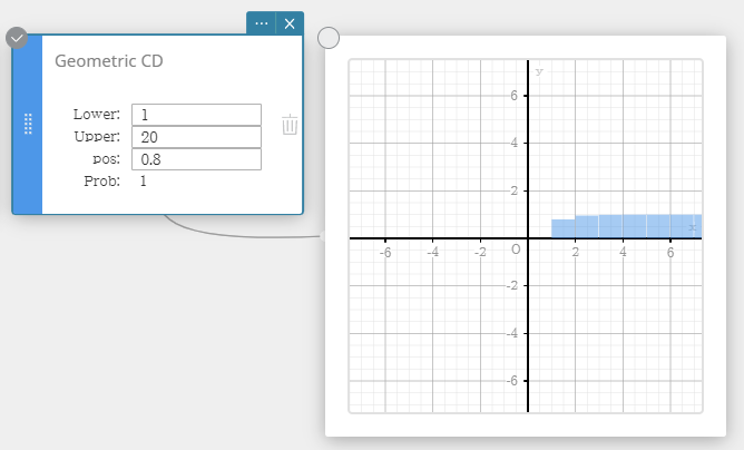 |
|
・Input Terms
・Output Terms
|
|
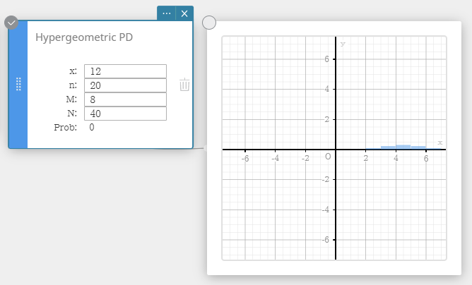
| Hypergeometric PD (Hypergeometric Distribution Probability) | |
|
Calculates the probability in a hypergeometric distribution that the success will occur on a specified trial. $$ prob = \cfrac{ {}_MC_x \times {}_{N-M}C_{n-x} }{ {}_NC_n } $$ |
 |
|
・Input Terms
・Output Terms
|
|
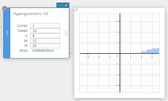
| Hypergeometric CD (Hypergeometric Cumulative Distribution) | |
|
Calculates the cumulative probability in a hypergeometric distribution that the success will occur on or before a specified trial. $$ prob = \sum_{i=Lower}^{Upper}\frac{ {}_MC_i \times {}_{N-M}C_{n-i} }{ {}_NC_n } $$ |
 |
|
・Input Terms
・Output Terms
|
|
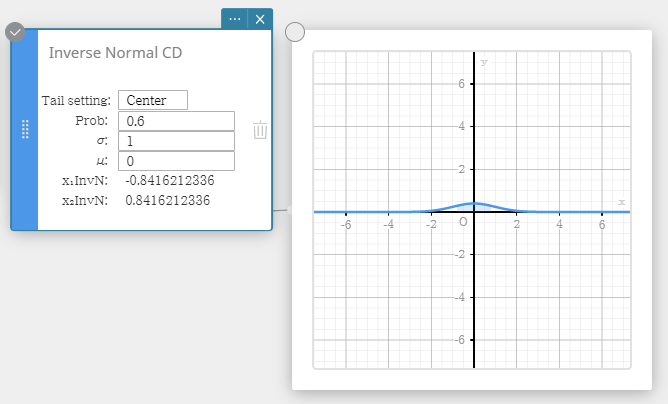
| Inverse Normal CD (Inverse Normal Cumulative Distribution) | |
|
Calculates the boundary value(s) of a normal cumulative probability distribution for specified values. Tail: Left $$ \int_{-\infty}^{\alpha}f(x)dx=p $$ Upper bound α is returned. Tail: Right $$ \int_{\alpha}^{+\infty}f(x)dx=p $$ Lower bound α is returned. Tail: Center $$ \int_{\alpha}^{\beta}f(x)dx=p \qquad \left( \mu=\cfrac{\alpha+\beta}{2} \right) $$ Lower bound α and upper bound β are returned. |
 |
|
・Input Terms
・Output Terms
|
|
| Inverse t CD (Inverse Student’s t Cumulative Distribution) | |
|
Calculates the lower bound value of a Student’s t cumulative probability distribution for specified values. $$ \int_{\alpha}^{+\infty}f(x)=p $$ |
 |
|
・Input Terms
・Output Terms
|
|
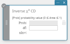
| Inverse χ2 CD (Inverse χ2 Cumulative Distribution) | |
|
Calculates the lower bound value of a χ2 cumulative probability distribution for specified values. $$ \int_{\alpha}^{+\infty}f(x)=p $$ |
 |
|
・Input Terms
・Output Terms
|
|
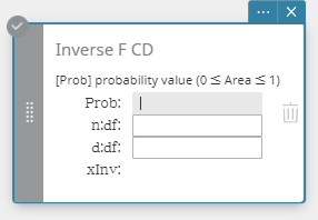
| Inverse F CD (Inverse F Cumulative Distribution) | |
|
Calculates the lower bound value of an F cumulative probability distribution for specified values. $$ \int_{\alpha}^{+\infty}f(x)=p $$ |
 |
|
・Input Terms
・Output Terms
|
|
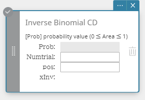
| Inverse Binomial CD (Inverse Binomial Cumulative Distribution) | |
|
Calculates the minimum number of trials of a binomial cumulative probability distribution for specified values. $$ \sum_{x=0}^{m}f(x)\ge prob $$ |
 |
|
・Input Terms
・Output Terms
|
|
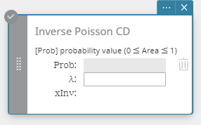
| Inverse Poisson CD (Inverse Poisson Cumulative Distribution) | |
|
Calculates the minimum number of trials of a Poisson cumulative probability distribution for specified values. $$ \sum_{x=0}^{m}f(x)\ge prob $$ |
 |
|
・Input Terms
・Output Terms
|
|
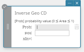
| Inverse Geo CD (Inverse Geometric Cumulative Distribution) | |
|
Calculates the minimum number of trials of a geometric cumulative probability distribution for specified values. $$ \sum_{x=0}^{m}f(x)\ge prob $$ |
 |
|
・Input Terms
・Output Terms
|
|
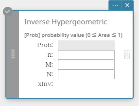
| Inverse Hypergeometric (Inverse Hypergeometric Cumulative Distribution) | |
|
Calculates the minimum number of trials of a hypergeometric cumulative probability distribution for specified values. $$ prob \le \sum_{i=0}^{X} \cfrac{ {}_MC_i \times {}_{N-M}C_{n-i} }{ {}_NC_n } $$ |
 |
|
・Input Terms
・Output Terms
|
|
4-11-6. Other Statistical Graphs
| Scatter Plot | |
|---|---|
| This plot compares the data accumulated ratio with a normal distribution accumulated ratio. If the scatter plot is close to a straight line, then the data is approximately normal. A departure from the straight line indicates a departure from normality. | 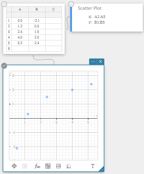 |
| Box & Whisker Plot | |
| This type of graph lets you see how a large number of data items are grouped within specific ranges. A box encloses all the data in an area from the first quartile ($Q1$) to the third quartile ($Q3$), with a line drawn at the median ($Med$). Lines (called whiskers) extend from either end of the box up to the minimum ($minX$) and maximum ($maxX$) of the data. | 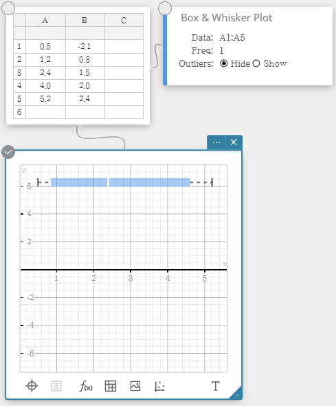 |
| Histogram | |
| A histogram shows the frequency (frequency distribution) of each data class as a rectangular bar. Classes are on the horizontal axis, while frequency is on the vertical axis. You can change the start value ($HStart$) and step value ($HStep$) of the histogram, if you want. | 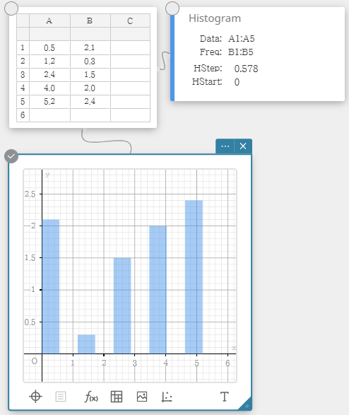 |
| Pie Chart | |
| You can draw a circle graph based on the data in a specific list. | 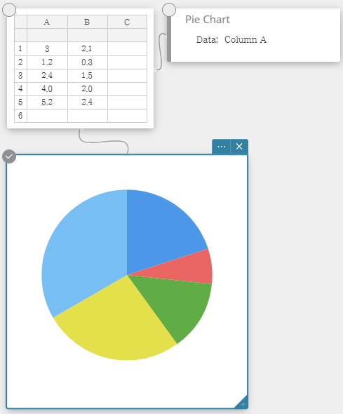 |
| Dot Plot | |
| The values in Column A (horizontal axis) represents bin numbers, while the values in Column B (vertical axis) represent the data point count in each bin. A dot is plotted for each data point in a bin. | 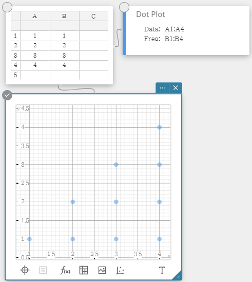 |