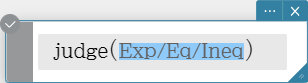
The following are the meanings of the abbreviations and punctuation used in the syntax descriptions in this section. Exp: Expression (Value, Variable, etc.) List: List Eq: Equation Mat: Matrix Ineq: All types of inequalities ($\small{{\rm a} \gt {\rm b},~ {\rm a} \geq {\rm b},~ {\rm a} \lt {\rm b},~ {\rm a} \leq {\rm b},~ {\rm a} \neq {\rm b}}$) Ineq$\small{\neq}$: Inequality $\small{{\rm a} \neq {\rm b}}$ only [ ]: You can omit the item(s) inside the brackets. { }: Select one of the items inside the braces. Some of the syntaxes in the following explanations indicate the following for parameters: Exp/Eq/Ineq/List/Mat These abbreviations mean that you can use any of the following as a parameter: expression, equation, inequality, list, or matrix.
Abbreviations and Punctuation Used in This Section
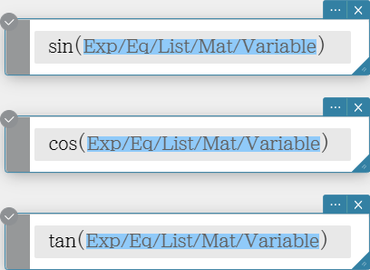
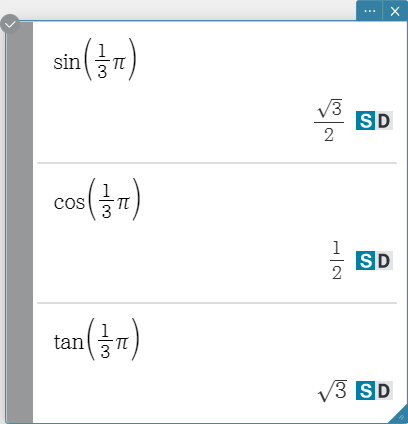
Trigonometric and Inverse Trigonometric Functions
sin, cos, tan
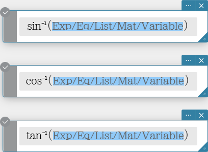
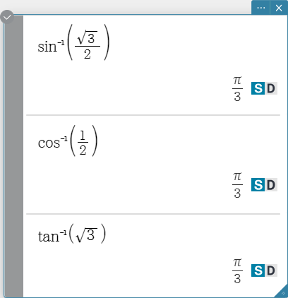
 sin\( ^{- 1}\), cos\( ^{- 1}\), tan\( ^{- 1}\)
Hyperbolic and Inverse Hyperbolic Functions
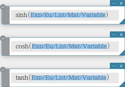
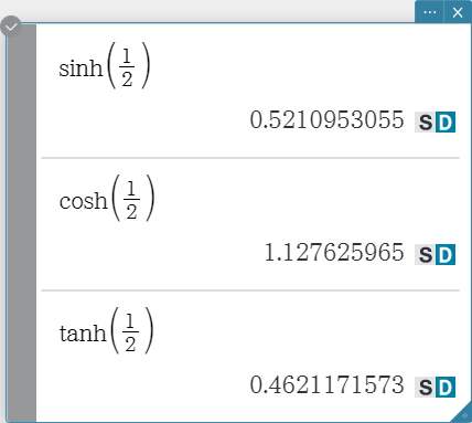
sinh, cosh, tanh
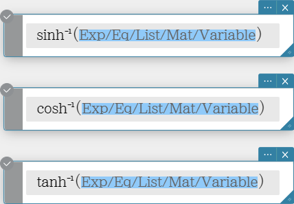
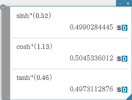
 sinh\( ^{- 1}\), cosh\( ^{- 1}\), tanh\( ^{- 1}\)
Angle Units
° r
Mixed Fraction
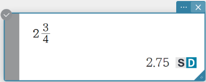
mixedFraction
Syntax: \( ■\frac □□ \)

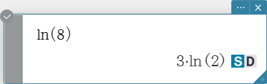
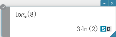
Logarithmic Function
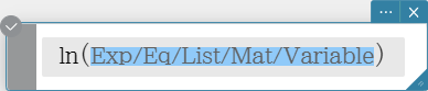
ln, log

Numeric Calculations
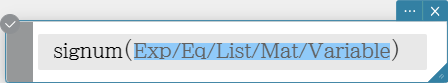
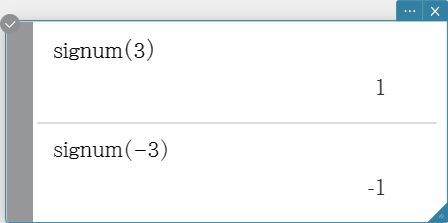
signum
signum returns –1 for a negative value, 1 for a positive value,
“Undefined” for 0, and \( \frac{A}{|A|} \) for an imaginary number.
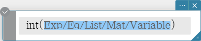
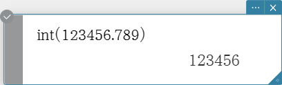
Int
Returns the integer part of a value.
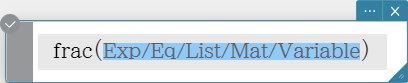
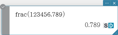
frac
Returns the decimal part of a value.
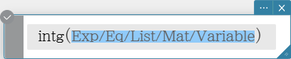
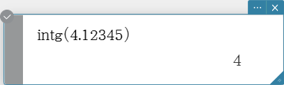
intg
Returns the largest integer that does not exceed a value.
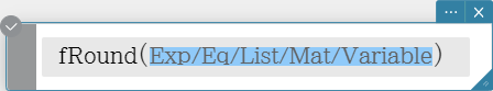
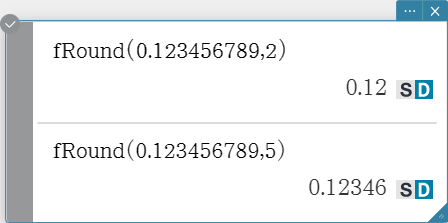
fRound
Rounds the decimal part of a value to the specified number of decimal places.
Syntax: fRound (Exp/Eq/List/Mat/Variable [ ) ]
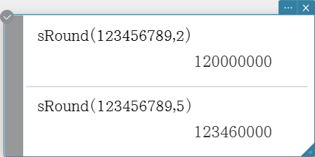
sRound
Rounds a value to the specified number of digits.
Syntax: sRound (Exp/Eq/List/Mat/Variable [ ) ]

Random Number Generator
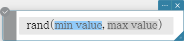
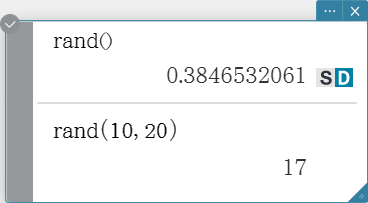
rand
Syntax: rand([a, b])
The “rand” function generates random numbers. If you do not specify an argument,
“rand” generates 10-digit decimal values 0 or greater and less than 1.
Specifying two integer values for the argument generates random numbers between them.

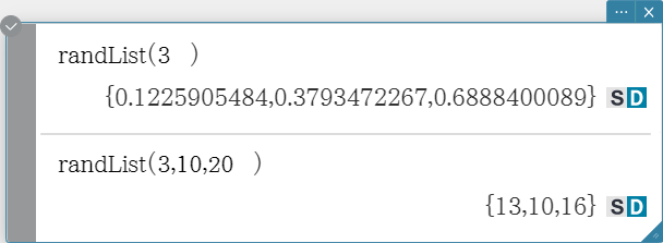
randList
Syntax: randList( n [, a, b])
- Omitting arguments “a” and “b” returns a list of n elements that contain decimal random values.
- Specifying arguments “a” and “b” returns a list of n elements that contain integer random values in the range of “a” through “b”.
- “n” must be a positive integer.
- The random numbers of each element are generated in accordance with “RandSeed” specifications.

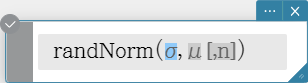
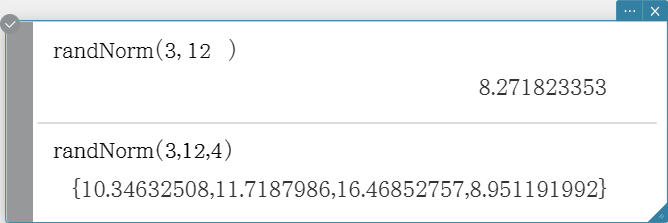
randNorm
The “randNorm” function generates a 10-digit normal random number based on a specified mean μ and standard deviation σ values. Syntax: randNorm(σ, μ [, n ])
- Omitting a value for “n” (or specifying 1 for “ n ”) returns the generated random number as-is.
- Specifying 2 or larger value for “n” returns the specified number of random values in list format.
- “n” must be a positive integer, and “σ” must be greater than 0.
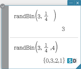
randBin
The “randBin” function generates binomial random numbers based on values specified for the number of trials n and probability P. Syntax: randBin( n, P [, m ])
- Omitting a value for “m” (or specifying 1 for “m”) returns the generated random number as-is.
- Specifying a 2 or larger value for “m” returns the specified number of random values in list format.
- “n” and “m” must be positive integers.

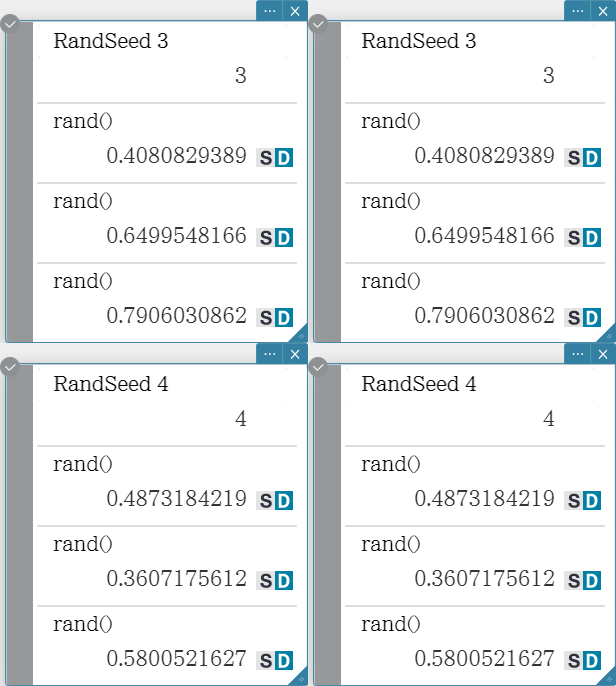
RandSeed
- You can specify an integer from 0 to 9 for the argument of this command. 0 specifies non-sequential random number generation. An integer from 1 to 9 uses the specified value as a seed for specification of sequential random numbers. The initial default argument for this command is 0.
- The numbers generated by the application immediately after you specify sequential random number generation always follow the same random pattern.

Integer Functions
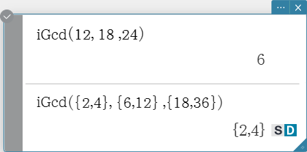
iGcd
Syntax: iGcd(Exp-1, Exp-2[, Exp-3…Exp-10)] (Exp-1 through Exp-10 all are integers.) iGcd(List-1, List-2[, List-3…List-10)] (All elements of List-1 through List-10 are integers.)
- The first syntax above returns the greatest common divisor for two to ten integers.
- The second syntax returns, in list format, the greatest common divisor (GCD) for each of the elements in two to ten lists. When the arguments are {a, b}, {c, d}, for example, a list will be returned showing the GCD for a and c, and for b and d.


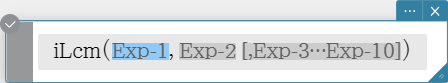
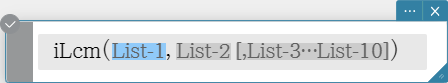
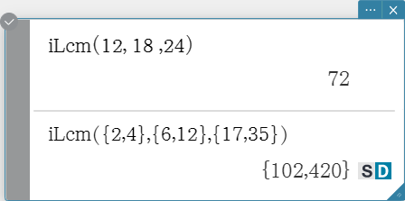
iLcm
Syntax: iLcm(Exp-1, Exp-2[, Exp-3…Exp-10)] (Exp-1 through Exp-10 all are integers.) iLcm(List-1, List-2[, List-3…List-10)] (All elements of List-1 through List-10 are integers.)
- The first syntax above returns the least common multiple for two to ten integers.
- The second syntax returns, in list format, the least common multiple (LCM) for each of the elements in two to ten lists. When the arguments are {a, b}, {c, d}, for example, a list will be returned showing the LCM for a and c, and for b and d.
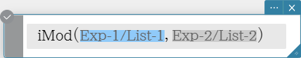
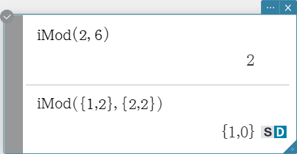
iMod
Syntax: iMod(Exp-1/List-1, Exp-2/List-2[)] (Exp-1, Exp-2 and all of the elements of List-1 and List-2 must be integers.)
- This function divides one or more integers by one or more other integers and returns the remainder(s).
Permutation and Combination
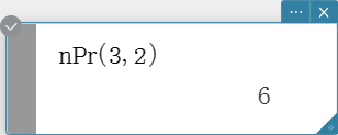
nPr
Syntax: nPr(n, r[)] (“n” and “r” must be positive integers.)
- Returns the total number of permutations where n is the total number of objects in the set and r is the number of objects chosen from the set.
\[ {}_n P_r = \frac{n!}{(n-r)!} \]

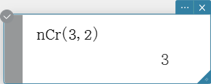
nCr
Syntax: nCr(n, r[)] (“n” and “r” must be positive integers.)
- Returns the total number of combinations where n is the total number of objects in the set and r is the number of objects chosen from the set.
\[ {}_n C_r = \frac{n!}{r!(n-r)!} \]

Other Functions
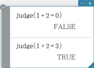
judge
The “judge” function returns TRUE when an expression is true, and FALSE when it is false.
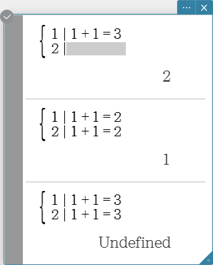
piecewise
The “piecewise” function returns one value when an expression is true,
and another value when the expression is false.
Syntax:
\[ \begin{cases} \lt \text{return value when true} \gt | \lt \text{condition expression} \gt \\
\lt \text{return value when false or indeterminate} \gt \end{cases} \]
or
\[ \begin{cases} \lt \text{return value when condition 1 is true} \gt | \lt \text{condition 1 expression}
\gt \\ \lt \text{return value when condition 2 is true} \gt | \lt \text{condition 2 expression}
\gt \end{cases} \]

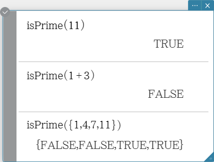
isPrime
The “isPrime” function determines whether the number provided as the argument is prime (returns TRUE) or not (returns FALSE). Syntax: isPrime(Exp/List[ ) ]
- Exp or all of the elements of List must be integers.

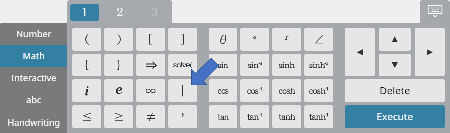
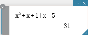
with Operator ( | )
The “with” ( | ) operator temporarily assigns a value to a variable. You can use the “with” operator in the following cases.
- To assign the value specified on the right side of | to the variable on the left side of |
- To limit or restrict the range of a variable on the left side of | in accordance with conditions provided on the right side of |
- Use the [Math] keyboard to input |.
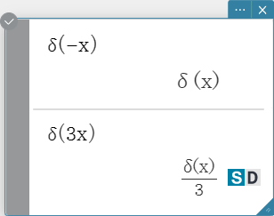
delta
“delta” is the Dirac Delta function. The delta function evaluates numerically as shown below.
\[ \delta(x) = \begin{cases} 0, x \neq 0 \\ \delta(x), x=0 \end{cases} \]
\( x \) : variable or number

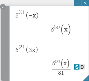
\(n\)th-delta
The \(n\)th-delta function is the \(n\)th differential of the delta function.
Syntax: \( δ^{(n)} (x) \)
\( x \) : variable or number
\( n \) : number of differentials

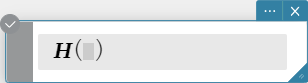
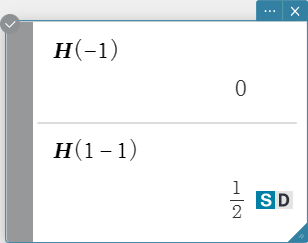
heaviside
“heaviside” is the command for the Heaviside function, which evaluates only to numeric expressions as shown below.
\[ H(x) = \begin{cases} 0, x<0 \\ \frac 12, x = 0 \\ 1, x>0 \end{cases} \]
\( x \) : variable or number
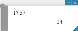
gamma
“gamma” is the command for the Gamma function.
Syntax: \( \Gamma (x) = \int_0^{+\infty} t^{x-1} e^{-t} dt \)
\( x \) : variable or number

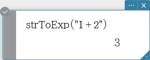
strToExp
Converts a string to an expression, and executes the expression.
Syntax: strToExp ("<string>")
Transformation
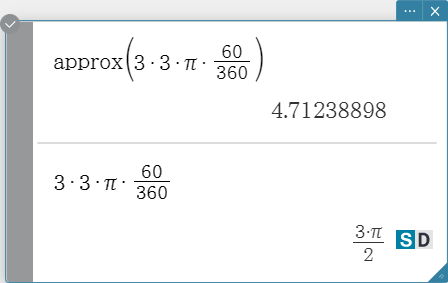
approx
Transforms an expression into a numerical approximation.
Syntax: approx (Exp/Eq/List/Mat/Variable [ ) ]

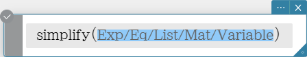
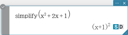
simplify
Simplifies an expression.
Syntax: simplify (Exp/Eq/List/Mat/Variable [ ) ]
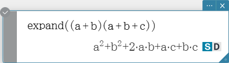
expand
Expands an expression.
Syntax: expand (Exp/Eq/List/Mat/Variable [ ) ]
expand (Exp,Variable [ ) ]


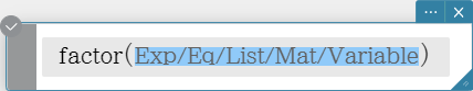
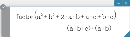
factor
Factors an expression.
Syntax: factor (Exp/Eq/List/Mat/Variable [ ) ]
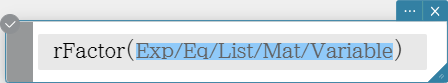
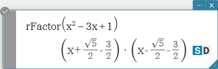
rFactor
Factors an expression up to its roots, if any.
Syntax: rFactor (Exp/Eq/List/Mat/Variable [ ) ] ]
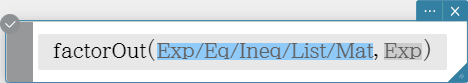
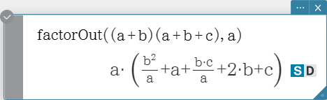
factorOut
Factors out an expression with respect to a specified factor.
Syntax: factorOut (Exp/Eq/Ineq/List/Mat, Exp [ ) ]
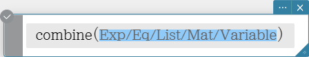
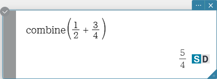
combine
Transforms multiple fractions into their common denominator equivalents and reduces them, if possible.
Syntax: combine (Exp/Eq/List/Mat/Variable [ ) ]
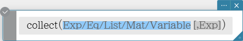
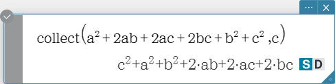
collect
Rearranges an expression with respect to a specific variable.
Syntax: collect (Exp/Eq/List/Mat/Variable[, Exp] [ ) ]
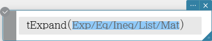
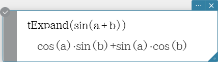
tExpand
Employs the sum and difference formulas to expand a trigonometric function.
Syntax: tExpand (Exp/Eq/Ineq/List/Mat [ ) ]
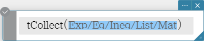
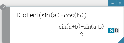
tCollect
Employs the product to sum formulas to transform the product of a trigonometric
function into an expression in the sum form.
Syntax: tCollect (Exp/Eq/Ineq/List/Mat [ ) ]
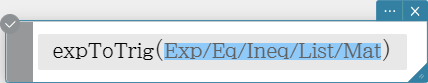
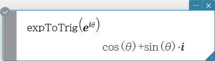
expToTrig
Transforms an exponent into a trigonometric or hyperbolic function.
Syntax: expToTrig (Exp/Eq/Ineq/List/Mat [ ) ]
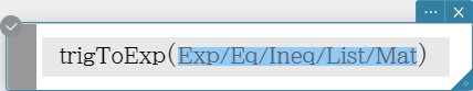
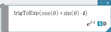
trigToExp
Transforms a trigonometric or hyperbolic function into exponential form.
Syntax: trigToExp (Exp/Eq/Ineq/List/Mat [ ) ]
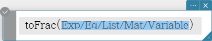
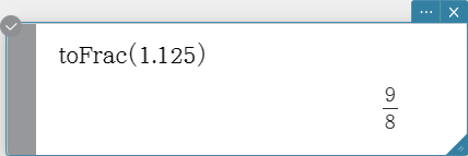
toFrac
Transforms a decimal value into its equivalent fraction value.
Syntax: toFrac (Exp/Eq/List/Mat/Variable [ ) ]
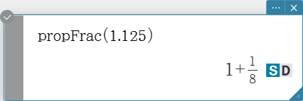
propFrac
Transforms a decimal value into its equivalent proper fraction value.
Syntax: propFrac (Exp/Eq/Ineq/List/Mat [ ) ]

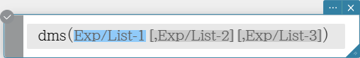
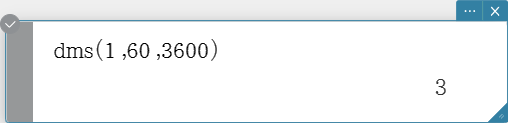
dms
Transforms a DMS format value into its equivalent degrees-only value.
Syntax: dms (Exp/List-1 [, Exp/List-2][, Exp/List-3] [ ) ]
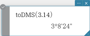
toDMS
Transforms a degrees-only value into its equivalent DMS format value.
Syntax: toDMS (Exp/List [ ) ]

Advanced
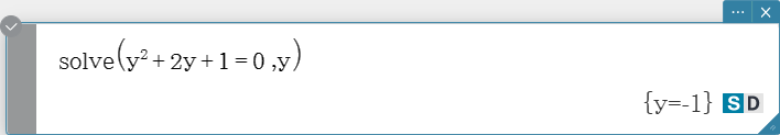
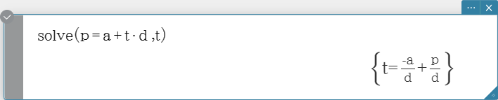
solve
Returns the solution of an equation or inequality. Syntax 1: solve(Exp/Eq/Ineq [, Variable] [ ) ]
- “$x$” is the default when you omit “[, Variable]”.

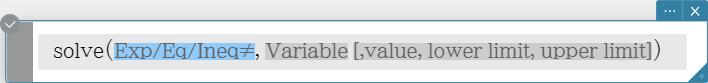
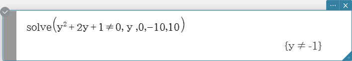
 Syntax 2: solve(Exp/Eq/Ineq$\small{\neq}$, Variable[, value, lower limit, upper limit] [ ) ]
- “value” is an initially estimated value.
- This command is valid only for equations and $\small{\neq}$ expressions when “value” and the items following it are included. In that case, this command returns an approximate value.
- A true value is returned when you omit “value” and the items following it. When, however, a true value cannot be obtained, an approximate value is returned for equations only based on the assumption that value = 0, lower limit = – ∞, and upper limit = ∞.
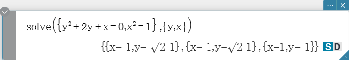
 Syntax 3: solve({Exp-1/Eq-1, ..., Exp-N/Eq-N}, {variable-1, ..., variable-N} [ ) ]
- When “Exp” is the first argument, the equation Exp = 0 is presumed.
 Syntax 4: You can solve for the relationship between two points, straight lines, planes, or
spheres by entering a vector equation inside the solve( command. Here we will
present four typical syntaxes for solving a vector equation using the solve( command.
In the syntaxes below, Vct-1 through Vct-6 are column vectors with three (or two) elements, and s, t, u and
v are parameters.
solve(Vct-1 + s * Vct-2 [= Vct-3, {variable-1}])
Syntax 4: You can solve for the relationship between two points, straight lines, planes, or
spheres by entering a vector equation inside the solve( command. Here we will
present four typical syntaxes for solving a vector equation using the solve( command.
In the syntaxes below, Vct-1 through Vct-6 are column vectors with three (or two) elements, and s, t, u and
v are parameters.
solve(Vct-1 + s * Vct-2 [= Vct-3, {variable-1}])
- If the right side of the equation (= Vct-3) is omitted in the above syntax, it is assumed that all of the elements on the right side are 0 vectors.
- Variables (variable 1 through variable 4) can be input into the elements of each vector (Vct-1 through Vct-6) in the above four syntaxes to solve for those variables.
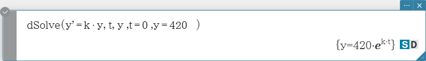
dSolve
Solves first, second or third order ordinary differential equations, or a system of first order differential equations.
Syntax: dSolve(Eq, independent variable, dependent variable [, initial condition-1, initial condition-2][, initial condition-3, initial condition-4][, initial condition-5, initial condition-6] [ ) ]
dSolve({Eq-1, Eq-2}, independent variable, {dependent variable-1, dependent variable-2} [, initial condition-1, initial condition-2, initial condition-3, initial condition-4] [ ) ]

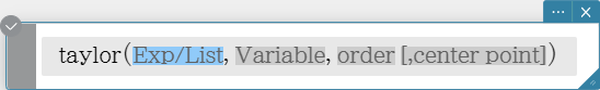
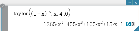
taylor
Finds a Taylor polynomial for an expression with respect to a specific variable.
Syntax: taylor (Exp/List, Variable, order [, center point] [ ) ]
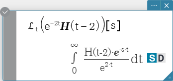
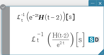
laplace, invLaplace
“laplace” is the command for the Laplace transform, and “invLaplace” is the command for
the inverse of Laplace transform.
Syntax: laplace \( ℒ_t (f(t))[s] \)
\( f(t) \): expression
\( t \): variable with respect to which the expression is transformed
\( s \): parameter of the transform
invLaplace \( ℒ_s^{-1} (L(s))[t] \)
\( L(s) \): expression
\( s \): variable with respect to which the expression is transformed
\( t \): parameter of the transform

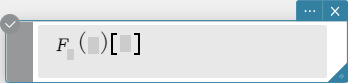
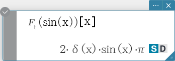
fourier, invFourier
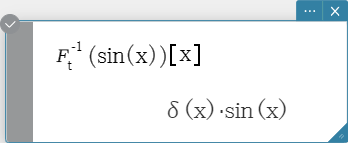
“fourier” is the command for the Fourier Transform, and “invFourier” is
the command for the inverse Fourier Transform.
Syntax: fourier \(Ϝ_x (f(x))[w] \)
invFourier \( Ϝ_w^{-1} (f(w))[x] \)
\( x \): variable with respect to which the expression is transformed
\( w \): parameter of the transform

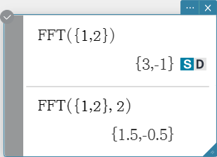
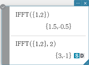
FFT, IFFT
“FFT” is the command for the fast Fourier Transform, and “IFFT” is the command for the inverse fast Fourier Transform.
2n data values are needed to perform FFT and IFFT. FFT and IFFT are calculated numerically.
Syntax: FFT(list) or FFT(list, m )
IFFT(list) or IFFT(list, m )


Calculation
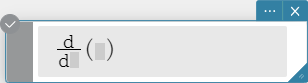
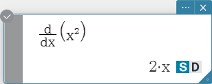
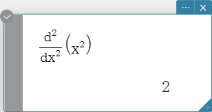
diff
Differentiates an expression with respect to a specific variable.
Syntax:
\( \frac{\mathrm d}{\mathrm d ■} □ \),
\( \frac{\mathrm d^□}{\mathrm d ■} □ \)

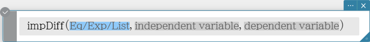
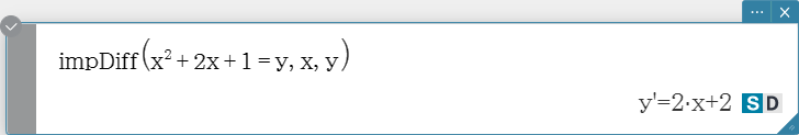
impDiff
Differentiates an equation or expression in implicit form with respect to a specific variable.
Syntax: impDiff(Eq/Exp/List, independent variable, dependent variable)
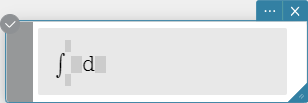
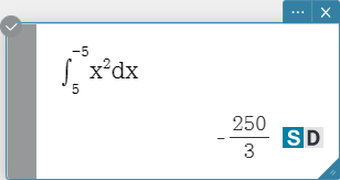
Integrate
Integrates an expression with respect to a specific variable.
Syntax: \( \int_□^□ ■ d□ \)
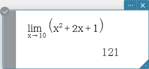
lim
Determines the limit of an expression.
Syntax: $$ \lim_{■ \to □} (■)$$

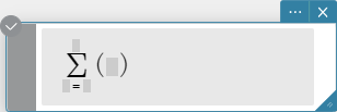
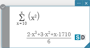
sum
Evaluates an expression at discrete variable values within a range, and then calculates a sum.
Syntax: \( \sum_{■=□}^{□} (⬚) \)
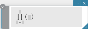
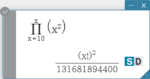
prod
Evaluates an expression at discrete variable values within a range, and then calculates a product.
Syntax: \( \prod_{■=□}^{□} ■ \)
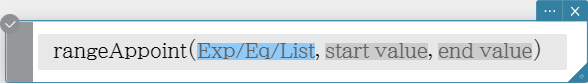
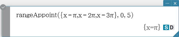
rangeAppoint
Finds an expression or value that satisfies a condition in a specified range.
Syntax: rangeAppoint (Exp/Eq/List, start value, end value [ ) ]
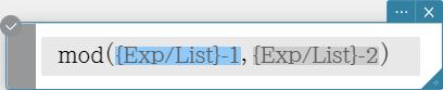
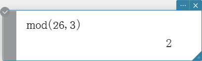
mod
Returns the remainder when one expression is divided by another expression.
Syntax: mod ({Exp/List} -1, {Exp/List} -2 [ ) ]
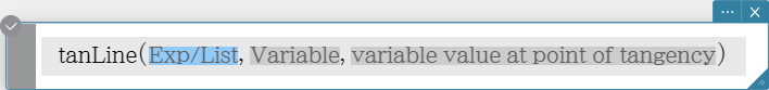
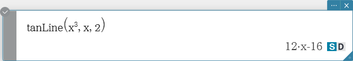
tanLine
Returns the right side of the equation for the tangent line (y = ‘expression’) to the curve at the specified point.
Syntax: tanLine (Exp/List, Variable, variable value at point of tangency [ ) ]
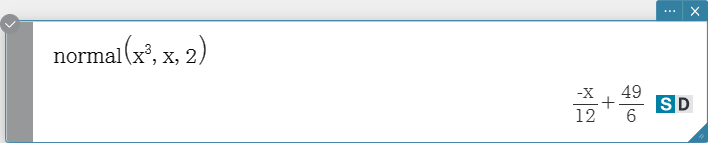
normal
Returns the right side of the equation for the line normal (y = ‘expression’)
to the curve at the specified point.
Syntax: normal (Exp/List, Variable, variable value at point of normal [ ) ]

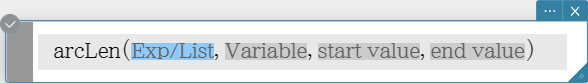
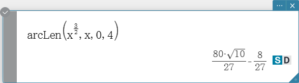
arcLen
Returns the arc length of an expression from a start value to an end value
with respect to a specified variable.
Syntax: arcLen (Exp/List, Variable, start value, end value [ ) ]
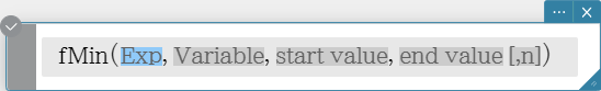
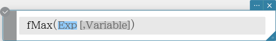
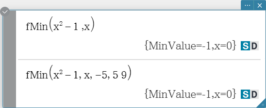
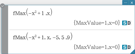
fMin, fMax
Returns the minimum (fMin) / the maximum (fMax) point in a specific range of a function. Syntax: fMin(Exp[, Variable] [ ) ] fMin(Exp, Variable, start value, end value[, n] [ ) ] fMax(Exp[, Variable] [ ) ] fMax(Exp, Variable, start value, end value[, n] [ ) ]
- “x” is the default when you omit “[, Variable]”.
- Negative infinity and positive infinity are the default when the syntax fMin(Exp[, Variable] [ ) ] or fMax(Exp[, Variable] [ ) ] is used.
- “n” is calculation precision, which you can specify as an integer in the range of 1 to 9. Using any value outside this range causes an error.
- This command returns an approximate value when calculation precision is specified for “n”.
- This command returns a true value when nothing is specified for “n”. If the true value cannot be obtained, however, this command returns an approximate value along with n = 4.
- Discontinuous points or sections that fluctuate widely can adversely affect precision or even cause an error.
- Inputting a larger number for “n” increases the precision of the calculation, but it also increases the amount of time required to perform the calculation.
- The value you input for the end point of the interval must be greater than the value you input for the start point. Otherwise an error occurs.


gcd
Returns the greatest common denominator of two expressions.
Syntax: gcd (Exp/List-1, Exp/List-2 [ ) ]

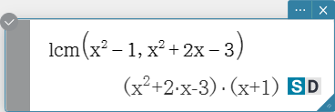
lcm
Returns the least common multiple of two expressions.
Syntax: lcm (Exp/List-1, Exp/List-2 [ ) ]
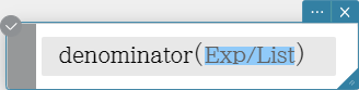
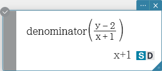
denominator
Extracts the denominator of a fraction.
Syntax: denominator (Exp/List [ ) ]
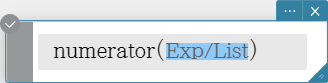
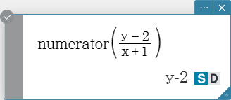
numerator
Extracts the numerator of a fraction.
Syntax: numerator (Exp/List [ ) ]
Complex
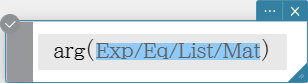
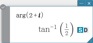
arg
Returns the argument of a complex number.
Syntax: arg (Exp/Eq/List/Mat [ ) ]
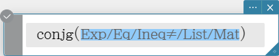
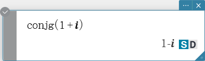
conjg
Returns the conjugate complex number.
Syntax: conjg (Exp/Eq/Ineq$\small{\neq}$/List/Mat [ ) ] (Ineq$\small{\neq}$: Real mode only)
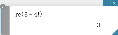
re
Returns the real part of a complex number.
Syntax: re (Exp/Eq/Ineq$\small{\neq}$/List/Mat [ ) ] (Ineq$\small{\neq}$: Real mode only)

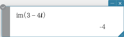
im
Returns the imaginary part of a complex number.
Syntax: im (Exp/Eq/Ineq$\small{\neq}$/List/Mat [ ) ] (Ineq$\small{\neq}$: Real mode only)

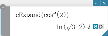
cExpand
Expands a complex expression to rectangular form (a + bi).
Syntax: cExpand (Exp/Eq/List/Mat [ ) ]
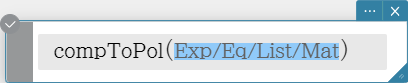
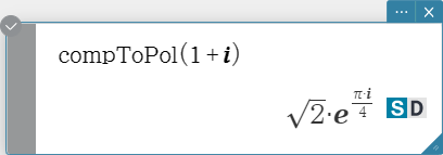
compToPol
Transforms a complex number into its polar form.
Syntax: compToPol (Exp/Eq/List/Mat [ ) ]
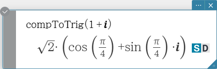
compToTrig
Transforms a complex number into its trigonometric/hyperbolic form.
Syntax: compToTrig (Exp/Eq/List/Mat [ ) ]

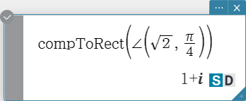
compToRect
Transforms a complex number into its rectangular form.
Syntax: compToRect ($∠(r, \theta)$ or $r \cdot e$^$(\theta \cdot i)$ form [ ) ]

List
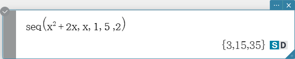
seq
Generates a list in accordance with a numeric sequence expression. Syntax: seq (Exp, Variable, start value, end value [, step size] [ ) ]
- “1” is the default when you omit “[, step size]”.
- The step size must be a factor of the difference between the start value and the end value.

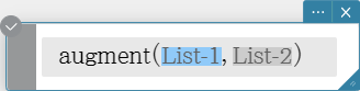
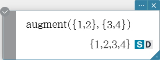
augment
Creates a new list by appending one list to another.
Syntax: augment (List-1, List-2 [ ) ]
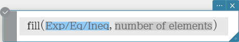
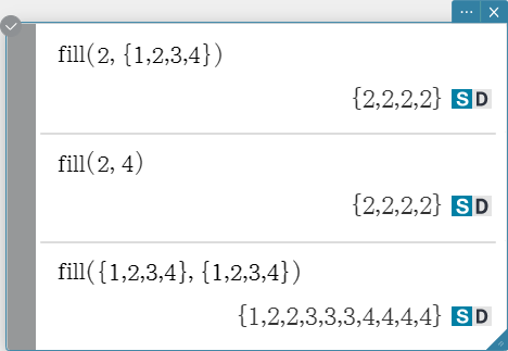
fill
Replaces the elements of a list with a specified value or expression. This command can also beused to create a new list whose elements all contain the same value or expression, or a new list inwhich the frequency of each element in the first list is determined by the corresponding element inthe second list.
Syntax: fill (Exp/Eq/Ineq, number of elements [ ) ]
fill (Exp/Eq/Ineq, List [ ) ]
fill (List, List [ ) ]


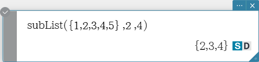
subList
Extracts a specific section of a list into a new list. Syntax: subList (List [, start number] [, end number] [ ) ]
- The leftmost element is the default when you omit “[, start number]”, and the rightmost element is the default when you omit “[, end number]”.

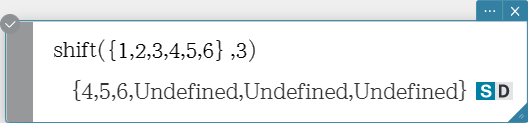
shift
Returns a list in which elements have been shifted to the right or left by a specific amount. Syntax: shift (List [, number of shifts] [ ) ]
- Specifying a negative value for “[, number of shifts]” shifts to the right, while a positive value shifts to the left.
- Right shift by one (–1) is the default when you omit “[, number of shifts]”.

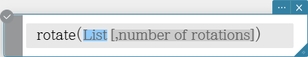
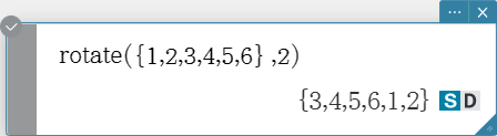
rotate
Returns a list in which the elements have been rotated to the right or to the left by a specific amount. Syntax: rotate (List [, number of rotations] [ ) ]
- Specifying a negative value for “[, number of rotations]” rotates to the right, while a positive value rotates to the left.
- Right rotation by one (–1) is the default when you omit “[, number of rotations]”.
sortA
Sorts the elements of the list into ascending order.
Syntax: sortA (List [ ) ]


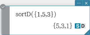
sortD
Sorts the elements of the list into descending order.
Syntax: sortD (List [ ) ]

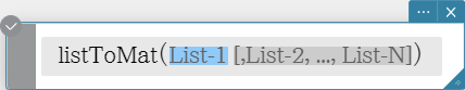
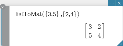
listToMat
Transforms lists into a matrix.
Syntax: listToMat (List-1 [, List-2, ..., List-N] [ ) ]
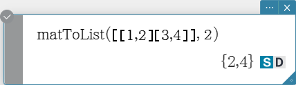
matToList
Transforms a specific column of a matrix into a list.
Syntax: matToList (Mat, column number [ ) ]

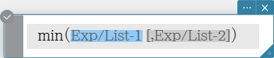
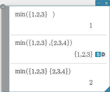
min
Returns the minimum value of an expression or the elements in a list.
Syntax: min (Exp/List-1[, Exp/List-2] [ ) ]
max
Returns the maximum value of an expression or the elements of a list.
Syntax: max (Exp/List-1[, Exp/List-2] [ ) ]


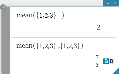
mean
Returns the mean of the elements in a list.
Syntax: mean (List-1[, List-2] [ ) ] (List-1: Data, List-2: Freq)

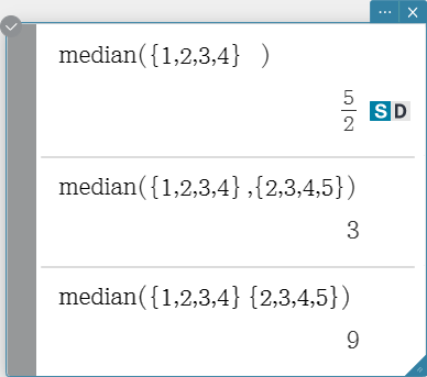
median
Returns the median of the elements in a list.
Syntax: median (List-1[, List-2] [ ) ] (List-1: Data, List-2: Freq)

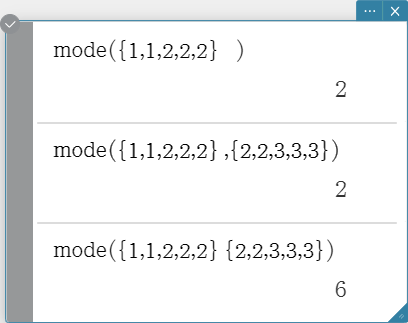
mode
Returns the mode of the elements in a list. If there are multiple modes, they are returned in a list.
Syntax: mode (List-1[, List-2] [ ) ] (List-1: Data, List-2: Freq)

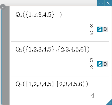
\( Q_1 \)
Returns the first quartile of the elements in a list.
Syntax: \( Q_1 \) (List-1[, List-2] [ ) ] (List-1: Data, List-2: Freq)

\( Q_3 \)
Returns the third quartile of the elements in a list.
Syntax: \( Q_3 \) (List-1[, List-2] [ ) ] (List-1: Data, List-2: Freq)


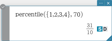
percentile
Finds the \(n\) th percentile point in a list.
Syntax: percentile (List, number)

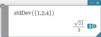
stdDev
Returns the sample standard deviation of the elements in a list.
Syntax: stdDev (List [ ) ]

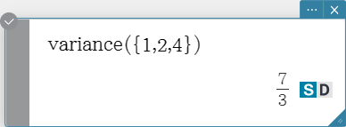
variance
Returns the sample variance of the elements in a list.
Syntax: variance (List [ ) ]

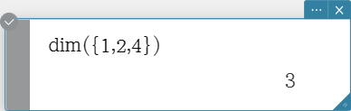
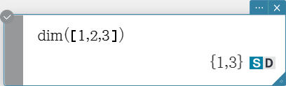
dim
Returns the dimension of a list.
Syntax: dim (List [ ) ]

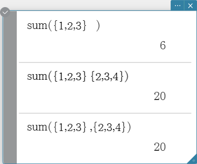
sum
Returns the sum of the elements in a list.
Syntax: sum (List-1[, List-2] [ ) ] (List-1: Data, List-2: Freq)

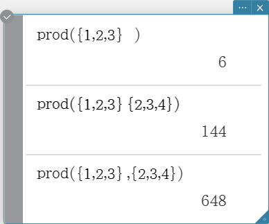
prod
Returns the product of the elements in a list.
Syntax: prod (List-1[, List-2] [ ) ] (List-1: Data, List-2: Freq)

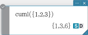
cuml
Returns the cumulative sums of the elements in a list.
Syntax: cuml (List [ ) ]

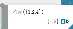
⊿list
Returns a list whose elements are the differences between two adjacent elements in another list.
Syntax: ⊿list (List [ ) ]

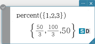
percent
Returns the percentage of each element in a list, the sum of which is assumed to be 100.
Syntax: percent (List [ ) ]

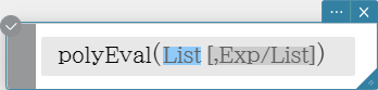
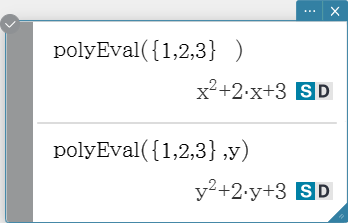
polyEval
Returns a polynomial arranged in the descending order of powers, so coefficients correspond sequentially to each element in the input list. Syntax: polyEval (List [, Exp/List] [ ) ]
- “$x$” is the default when you omit “[, Exp/List]”.
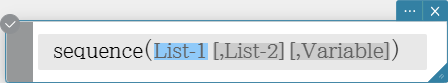
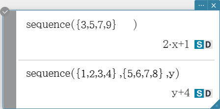
sequence
Returns the lowest-degree polynomial that represents the sequence expressed by the input list. When there are two lists, this command returns a polynomial that maps each element in the first list to its corresponding element in the second list. Syntax: sequence (List-1[, List-2] [, Variable] [ ) ]
- “$x$” is the default when you omit “[, Variable]”.
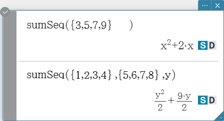
sumSeq
Finds the lowest-degree polynomial that represents the sequence expressed by the input list and returns the sum of the polynomial. When there are two lists, this command returns a polynomial that maps each element in the first list to its corresponding element in the second list, and returns the sum of the polynomial. Syntax: sumSeq (List-1[, List-2] [, Variable] [ ) ]
- “$x$” is the default when you omit “[, Variable]”.

Matrix
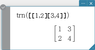
trn
Returns a transposed matrix.
Syntax: trn (Mat [ ) ]

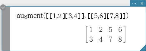
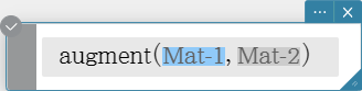
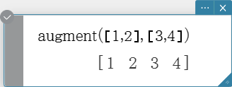
augment
Returns a matrix that combines two other matrices.
Syntax: augment (Mat-1, Mat-2 [ ) ]

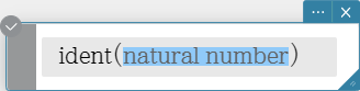
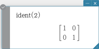
ident
Creates an identity matrix.
Syntax: ident (natural number [ ) ]
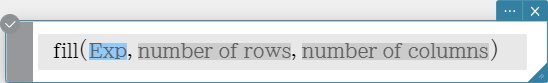
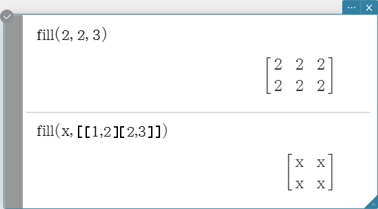
fill
Creates a matrix with a specific number of rows and columns, or replaces the elements of a matrix with a specific expression.
Syntax: fill (Exp, number of rows, number of columns [ ) ]
fill (Exp, Mat [ ) ]

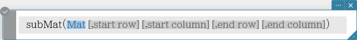
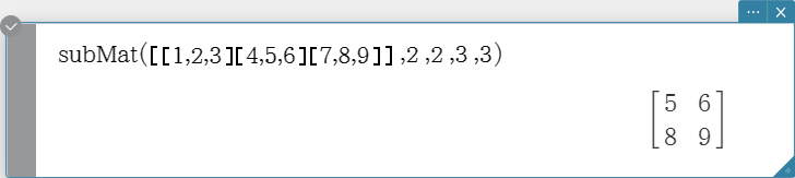
subMat
Extracts a specific section of a matrix into a new matrix. Syntax: subMat (Mat [, start row] [, start column] [, end row] [, end column] [ ) ]
- “1” is the default when you omit “[, start row]” and “[, start column]”.
- The last row number is the default when you omit “[, end row]”.
- The last column number is the default when you omit “[, end column]”.
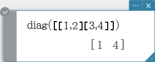
diag
Returns a one-row matrix containing the elements from the main diagonal of a square matrix.
Syntax: diag (Mat[ ) ]

listToMat
Transforms lists into a matrix.
Syntax: listToMat (List-1 [, List-2, ..., List-N] [ ) ]
matToList
Transforms a specific column of a matrix into a list.
Syntax: matToList (Mat, column number [ ) ]
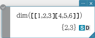
dim
Returns the dimensions of a matrix as a two-element list {number of rows, number of columns}.
Syntax: dim (Mat [ ) ]

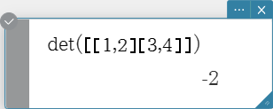
det
Returns the determinant of a square matrix.
Syntax: det (Mat [ ) ]

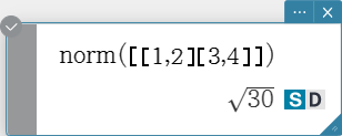
norm
Returns the Frobenius norm of the matrix.
Syntax: norm (Mat [ ) ]

rank
Finds the rank of matrix.
The rank function computes the rank of a matrix by performing Gaussian elimination on the rows of the given matrix. The rank of matrix A is the number of non-zero rows in the resulting matrix.
Syntax: rank (Mat [ ) ]
![]()
![]()
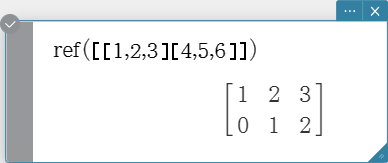
ref
Returns the row echelon form of a matrix.
Syntax: ref (Mat [ ) ]

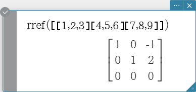
rref
Returns the reduced row echelon form of a matrix.
Syntax: rref (Mat [ ) ]

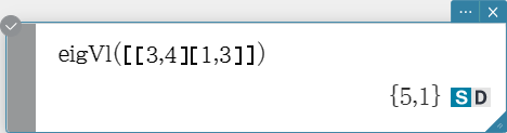
eigVl
Returns a list that contains the eigenvalue(s) of a square matrix.
Syntax: eigVl (Mat [ ) ]

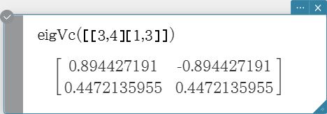
eigVc
Returns a matrix in which each column represents an eigenvector of a square matrix.
- Since an eigenvector usually cannot be determined uniquely, it is standardized as follows to its norm, which is 1:

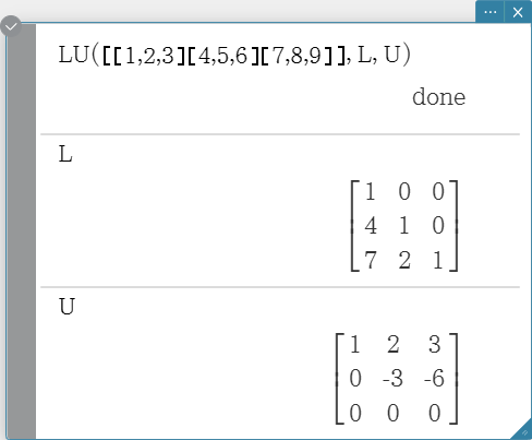
LU
Returns the LU decomposition of a square matrix. Syntax: LU (Mat, lVariableMem, uVariableMem [ ) ]
- The lower matrix is assigned to the first variable L, while the upper matrix is assigned to the second variable U.

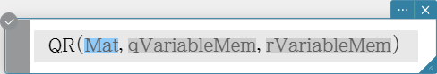
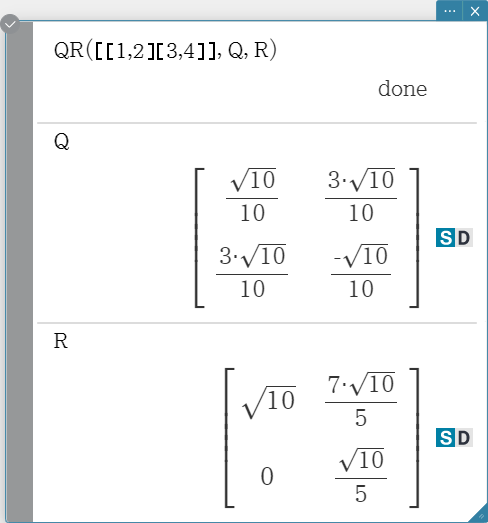
QR
Returns the QR decomposition of a square matrix. Syntax: QR (Mat, qVariableMem, rVariableMem [ ) ] Example: To obtain the QR decomposition of the matrix [[1, 2] [3, 4]]
- The unitary matrix is assigned to variable Q, while the upper triangular matrix is assigned to variable R.
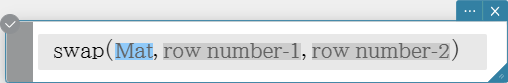
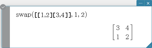
swap
Swaps two rows of a matrix.
Syntax: swap (Mat, row number-1, row number-2 [ ) ]
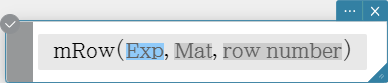
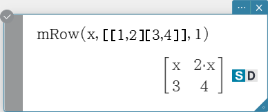
mRow
Multiplies the elements of a specific row in a matrix by a specific expression.
Syntax: mRow (Exp, Mat, row number [ ) ]
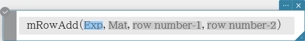
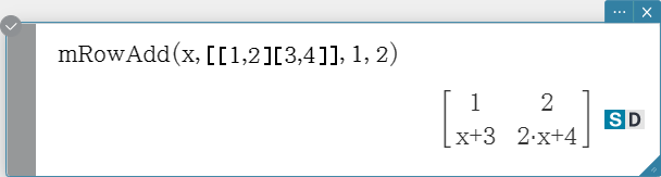
mRowAdd
Multiplies the elements of a specific row in a matrix by a specific expression, and then adds the result to another row.
Syntax: mRowAdd (Exp, Mat, row number-1, row number-2 [ ) ]
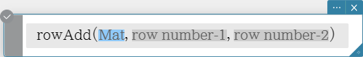
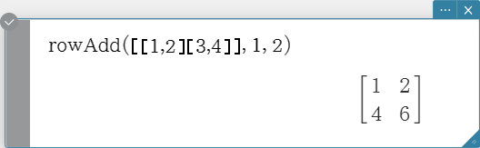
rowAdd
Adds a specific matrix row to another row.
Syntax: rowAdd (Mat, row number-1, row number-2 [ ) ]
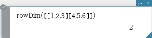
rowDim
Returns the number in rows in a matrix.
Syntax: rowDim (Mat [ ) ]

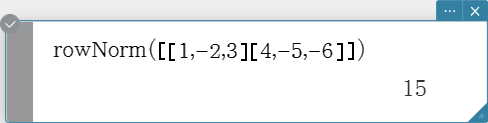
rowNorm
Calculates the sums of the absolute values of the elements of each row of a matrix, and returns the maximum value of the sums.
Syntax: rowNorm (Mat [ ) ]

colDim
Returns the number of columns in a matrix.
Syntax: colDim (Mat [ ) ]


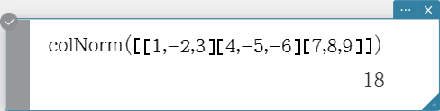
colNorm
Calculates the sums of the absolute values of the elements of each column of a matrix, and returns the maximum value of the sums.
Syntax: colNorm (Mat [ ) ]

Vector
- A vector is handled as a 1 $\times$ N matrix or N $\times$ 1 matrix.
- A vector in the form of 1 $\times$ N can be entered as [……] or [[……]].
- Example: [1, 2], [[1, 2]]
- Vectors are considered to be in rectangular form unless ∠() is used to indicate an angle measure.
augment
Returns an augmented vector [Mat-1 Mat-2].
Syntax: augment (Mat-1, Mat-2 [ ) ]
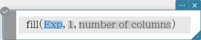
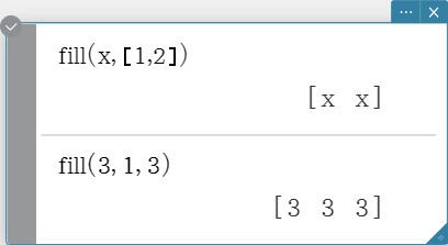
fill
Creates a vector that contains a specific number of elements, or replaces the elements of a vector with a specific expression.
Syntax: fill (Exp, Mat [ ) ]
fill (Exp, 1, number of columns [ ) ]

dim
Returns the dimension of a vector.
Syntax: dim (Mat [ ) ]

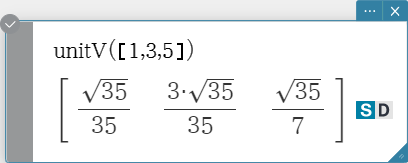
unitV
Normalizes a vector. Syntax: unitV (Mat [ ) ]
- This command can be used with a 1 $\times$ N or N $\times$ 1 matrix only.

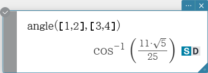
angle
Returns the angle formed by two vectors. Syntax: angle (Mat-1, Mat-2 [ ) ]
- This command can be used with a 1 $\times$ N or N $\times$ 1 matrix only.

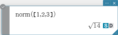
norm
Returns the norm of a vector.
Syntax: norm (Mat [ ) ]

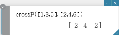
crossP
Returns the cross product of two vectors. Syntax: crossP (Mat-1, Mat-2 [ ) ]
- This command can be used with a 1 $\times$ N or N $\times$ 1 matrix only (N = 2, 3).
- A two-element matrix [a, b] or [[a], [b]] is automatically converted into a three-element matrix [a, b, 0] or [[a], [b], [0]].

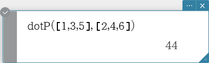
dotP
Returns the dot product of two vectors. Syntax: dotP (Mat-1, Mat-2 [ ) ]
- This command can be used with a 1 $\times$ N or N $\times$ 1 matrix only.

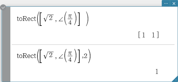
toRect
Returns an equivalent rectangular form $[\ x\ y\ ]$ or $[\ x\ y\ z\ ]$. Syntax: toRect (Mat [, natural number] [ ) ]
- This command can be used with a 1 $\times$ N or N $\times$ 1 matrix only (N = 2, 3).
- This command returns “x” when “natural number” is 1, “y” when “natural number” is 2, and “z” when “natural number” is 3.
- This command returns a rectangular form when you omit “natural number”.

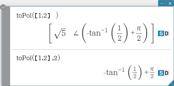
toPol
Returns an equivalent polar form $[\ r\ ∠\theta\ ]$. Syntax: toPol (Mat [, natural number] [ ) ]
- This command can be used with a 1 $\times$ 2 or 2 $\times$ 1 matrix only.
- This command returns “$r$” when “natural number” is 1, and “$\theta$” when “natural number” is 2.
- This command returns a polar form when you omit “natural number”.

toSph
Returns an equivalent spherical form $[\ \rho\ ∠\theta\ \ ∠\phi\ ]$. Syntax: toSph (Mat [, natural number] [ ) ]
- This command can be used with a 1 $\times$ 3 or 3 $\times$ 1 matrix only.
- This command returns “$\rho$” when “natural number” is 1, “$\theta$” when “natural number” is 2, and “$\phi$” when “natural number” is 3.
- This command returns a spherical form when you omit “natural number”.


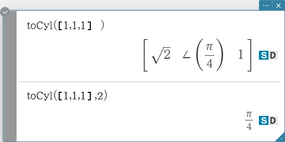
toCyl
Returns an equivalent cylindrical form $[\ r\ ∠\theta\ \ z\ ]$. Syntax: toCyl (Mat [, natural number] [ ) ]
- This command can be used with a 1 $\times$ 3 or 3 $\times$ 1 matrix only.
- This command returns “$r$” when “natural number” is 1, “$\theta$” when “natural number” is 2, and “$z$” when “natural number” is 3.
- This command returns a cylindrical form when you omit “natural number”.

Equation/Inequality
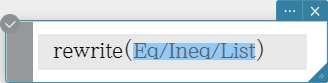
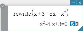
rewrite
Moves the right side elements of an equation or inequality to the left side.
Syntax: rewrite (Eq/Ineq/List [ ) ]
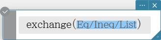
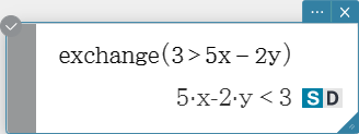
exchange
Swaps the right-side and left-side elements of an equation or inequality.
Syntax: exchange (Eq/Ineq/List [ ) ]
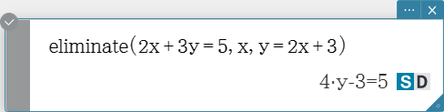
eliminate
Solves one equation with respect to a variable, and then replaces the same variable in another expression with the obtained result.
Syntax: eliminate (Eq/Ineq/List-1, Variable, Eq-2 [ ) ]

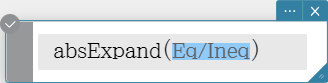
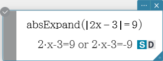
absExpand
Divides an absolute value expression into formulas without absolute value.
Syntax: absExpand (Eq/Ineq [ ) ]
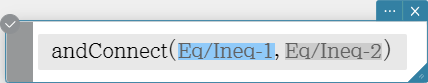
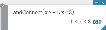
andConnect
Combines two equations or inequalities into a single expression.
Syntax: andConnect (Eq/Ineq-1, Eq/Ineq-2 [ ) ]
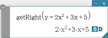
getRight
Extracts the right-side elements of an equation or inequality.
Syntax: getRight (Eq/Ineq/List [ ) ]

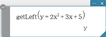
getLeft
Extracts the left-side elements of an equation or inequality.
Syntax: getLeft (Eq/Ineq/List [ ) ]

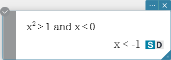
and
Returns the result of the logical AND of two expressions.
Syntax: Exp/Eq/Ineq/List-1 and Exp/Eq/Ineq/List-2

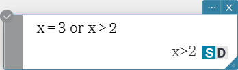
or
Returns the result of the logical OR of two expressions.
Syntax: Exp/Eq/Ineq/List-1 or Exp/Eq/Ineq/List-2

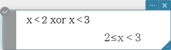
xor
Returns the logical exclusive OR of two expressions.
Syntax: Exp/Eq/Ineq/List-1 xor Exp/Eq/Ineq/List-2

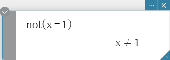
not
Returns the logical NOT of an expression.
Syntax: not(Exp/Eq/Ineq/List [ ) ]

Assistant
Note that the following commands are valid in the Assistant mode only. For more information on the Assistant mode see “2-14. Configuring Calculation Settings”.
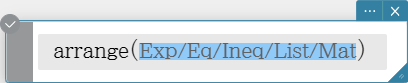
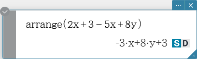
arrange
Combines common terms in an expression and returns the result arranged in descending sequence.
Syntax: arrange (Exp/Eq/Ineq/List/Mat [ ) ]
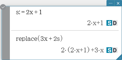
replace
Replaces the variable in an expression, equation or inequality with the value assigned to a variable using the “store” command.
Syntax: replace (Exp/Eq/Ineq/List/Mat [ ) ]

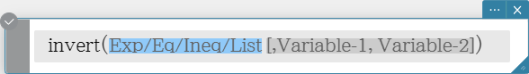
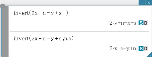
invert
Inverts two variables in an expression. Syntax: invert (Exp/Eq/Ineq/List [, Variable-1, Variable-2] [ ) ]
- x and y are inverted when variables are not specified.
Distribution/Inverse Distribution
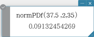
normPDf
Returns the normal probability density for a specified value. Syntax: normPDf (x[, σ, μ)]
- When σ and μ are skipped, σ = 1 and μ = 0 are used.

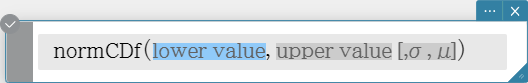
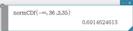
normCDf
Returns the cumulative probability of a normal distribution between a lower bound and an upper bound. Syntax: normCDf (lower value, upper value[, σ, μ)]
- When σ and μ are skipped, σ = 1 and μ = 0 are used.
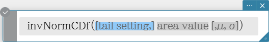
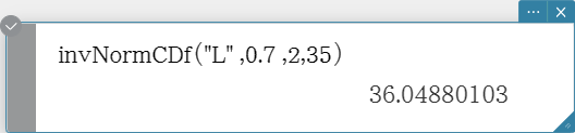
invNormCDf
Returns the boundary value(s) of a normal cumulative distribution probability for specified values. Syntax: invNormCDf ([tail setting, ]area value[, σ, μ)]
- When σ and μ are skipped, σ = 1 and μ = 0 are used.
- “tail setting” displays the probability value tail specification, and Left, Right, or Center can be specified. Enter the following values or letters to specify:
Left: −1, “L”, or “l” Center: 0, “C”, or “c” Right: 1, “R”, or “r”
When input is skipped, “Left” is used. - When “tail setting” is Center, the lower bound value is returned.
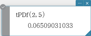
tPDf
Returns the Student’s t probability density for a specified value.
Syntax: tPDf (x, df [ ) ]
Calculation Result Output: prob

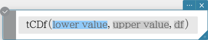
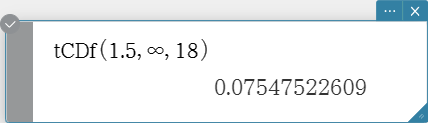
tCDf
Returns the cumulative probability of a Student’s t distribution between a lower bound and an upper bound.
Syntax: tCDf (lower value, upper value, df [ ) ]
Calculation Result Output: prob, tLow, tUp
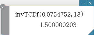
invTCDf
Returns the lower bound value of a Student’s t cumulative distribution probability for specified values.
Syntax: invTCDf (prob, df [ ) ]
Calculation Result Output: xInv

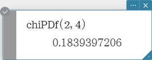
chiPDf
Returns the \( χ^2 \) probability density for specified values.
Syntax: chiPDf (x, df [ ) ]
Calculation Result Output: prob

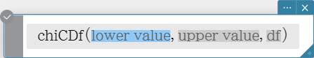
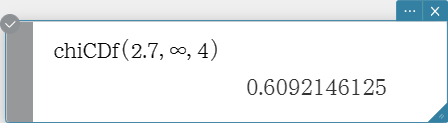
chiCDf
Returns the cumulative probability of a \( χ^2 \) distribution between a lower bound and an upper bound.
Syntax: chiCDf (lower value, upper value, df [ ) ]
Calculation Result Output: prob
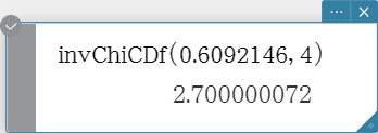
invChiCDf
Returns the lower bound value of a \( χ^2 \) cumulative distribution probability for specified values.
Syntax: invChiCDf (prob, df [ ) ]
Calculation Result Output: xInv

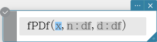
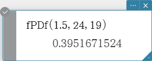
fPDf
Returns the F probability density for a specified value.
Syntax: fPDf (x, n:df, d:df [ ) ]
Calculation Result Output: prob
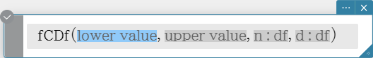
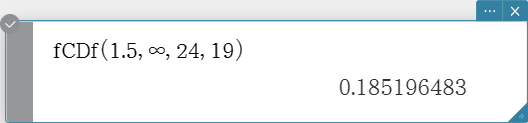
fCDf
Returns the cumulative probability of an F distribution between a lower bound and an upper bound.
Syntax: fCDf (lower value, upper value, n:df, d:df [ ) ]
Calculation Result Output: prob
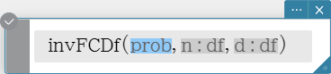
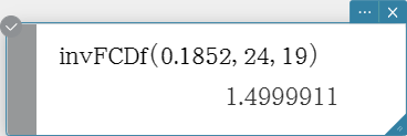
invFCDf
Returns the lower bound value of an F cumulative distribution probability for specified values.
Syntax: invFCDf (prob, n:df, d:df [ ) ]
Calculation Result Output: xInv
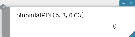
binomialPDf
Returns the probability in a binomial distribution that the success will occur on a specified trial.
Syntax: binomialPDf (x, numtrial value, pos [ ) ]
Calculation Result Output: prob

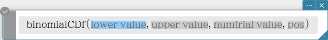
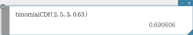
binomialCDf
Returns the cumulative probability in a binomial distribution that the success will occur between specified lower value and upper value.
Syntax: binomialCDf (lower value, upper value, numtrial value, pos [ ) ]
Calculation Result Output: prob
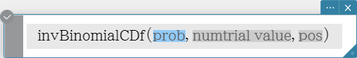
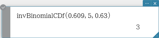
invBinomialCDf
Returns the minimum number of trials of a binomial cumulative probability distribution for specified values.
Syntax: invBinomialCDf (prob, numtrial value, pos [ ) ]
Calculation Result Output: xInv, *xInv
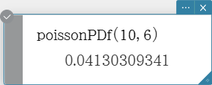
poissonPDf
Returns the probability in a Poisson distribution that the success will occur on a specified trial.
Syntax: poissonPDf (x, λ [ ) ]
Calculation Result Output: prob

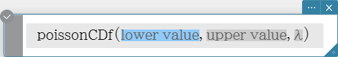
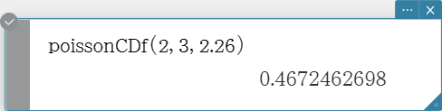
poissonCDf
Returns the cumulative probability in a Poisson distribution that the success will occur between specified lower value and upper value.
Syntax: poissonCDf (lower value, upper value, λ [ ) ]
Calculation Result Output: prob
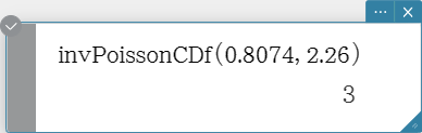
invPoissonCDf
Returns the minimum number of trials of a Poisson cumulative probability distribution for specified values.
Syntax: invPoissonCDf (prob, λ [ ) ]
Calculation Result Output: xInv, *xInv

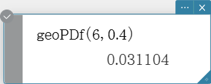
geoPDf
Returns the probability in a geometric distribution that the success will occur on a specified trial.
Syntax: geoPDf (x, pos [ ) ]
Calculation Result Output: prob

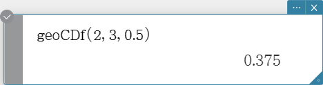
geoCDf
Returns the cumulative probability in a geometric distribution that the success will occur between specified lower value and upper value.
Syntax: geoCDf (lower value, upper value, pos [ ) ]
Calculation Result Output: prob

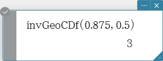
invGeoCDf
Returns the minimum number of trials of a geometric cumulative probability distribution for specified values.
Syntax: invGeoCDf (prob, pos [ ) ]
Calculation Result Output: xInv, *xInv

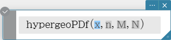
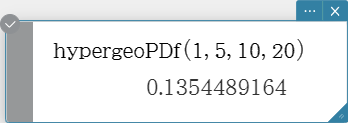
hypergeoPDf
Returns the probability in a hypergeometric distribution that the success will occur on a specified trial.
Syntax: hypergeoPDf (x, n, M, N [ ) ]
($n$: Number of elements extracted from population、 $M$: Number of successes in population、 $N$: Number of population elements)
Calculation Result Output: prob
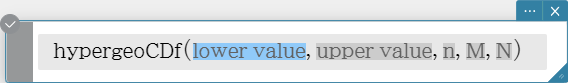
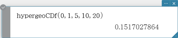
hypergeoCDf
Returns the cumulative probability in a hypergeometric distribution that the success will occur between specified lower value and upper value.
Syntax: hypergeoCDf (lower value, upper value, n, M, N [ ) ]
($n$: Number of elements extracted from population、 $M$: Number of successes in population、 $N$: Number of population elements)
Calculation Result Output: prob
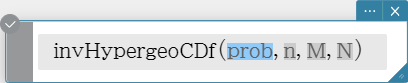
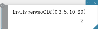
invHypergeoCDf
Returns the minimum number of trials of a hypergeometric cumulative distribution for specified values.
Syntax: invHypergeoCDf (prob, n, M, N [ ) ]
($n$: Number of elements extracted from population、 $M$: Number of successes in population、 $N$: Number of population elements)
Calculation Result Output: xInv, *xInv