3. Graphing and Numerical Table Creation
- 3-1. Basic Graphing Operations
- 3-2. Drawing Multiple Graphs
- 3-3. Graphing a Rectangular Coordinate Equation (y=, x=)
- 3-4. Graphing a Polar Coordinate Equation (r=)
- 3-5. Graphing a Parametric Function
- 3-6. Graphing an Inequality
- 3-7. Drawing Circle, Elliptic, and Hyperbolic Graphs
- 3-8. Using a List of Values to Draw Multiple Graphs
- 3-9. Specifying a Range to Draw a Graph
- 3-10. Using Trace
- 3-11. Basic Graph Analysis Operations
- 3-12. Creating a Table
- 3-13. Editing a Table
- 3-14. Using a Slider
- 3-15. Configuring Graph Display Settings
- 3-16. Zooming a Graph
- 3-17. Panning a Graph
- 3-18. Changing the color of a Graph
- 3-19. Hiding a Graph
- 3-20. Displaying a Background Image
- 3-21. Plot Function
- 3-22. Inputting Text
- 3-23. Determining the Integral Value and Area of a Region
- 3-24. Drawing a Line Tangent or Normal to a Graph
3-1. Basic Graphing Operations
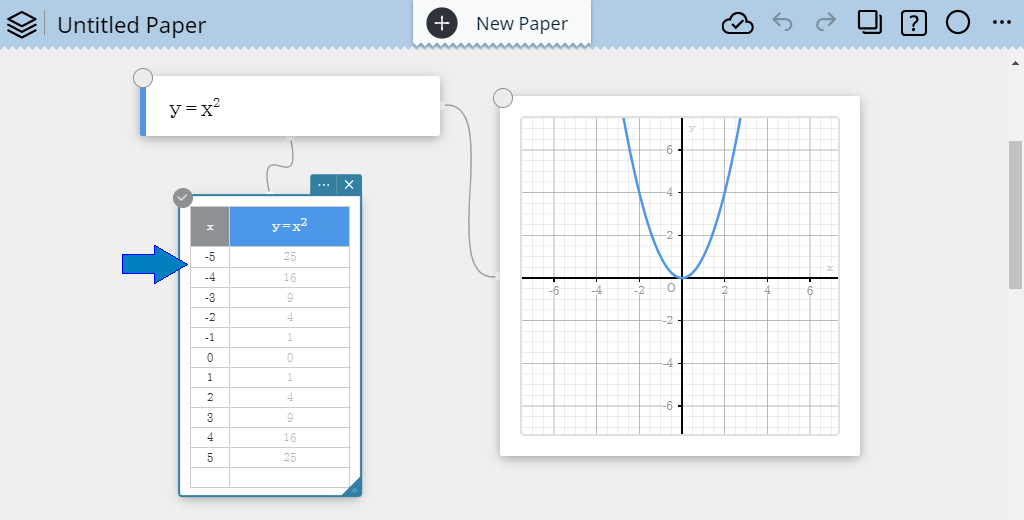
3-1-1. To draw a graph and create a numerical table
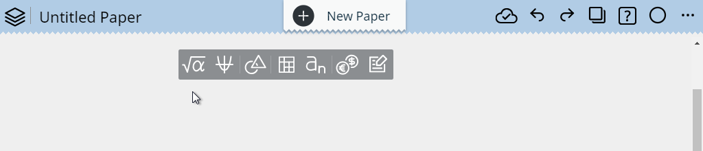
1. Click anywhere on the Paper.
• This displays the Sticky Note menu.
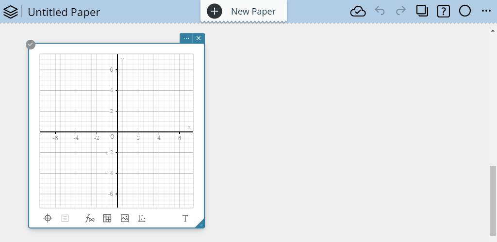
2. Click  .
.
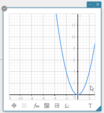
• This displays a Graph Sticky Note.
3. At the bottom of the Graph Sticky Note, click  .
.
• This displays a Graph Function Sticky Note.
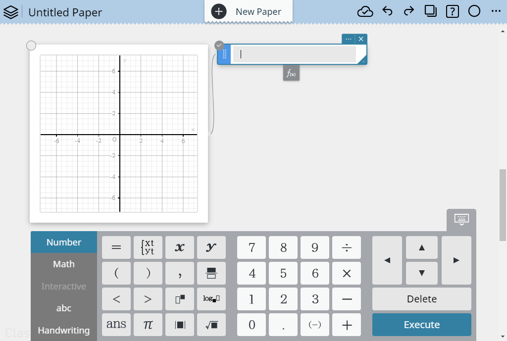
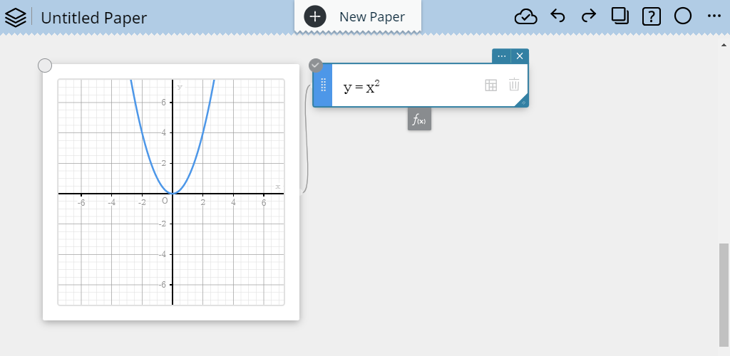
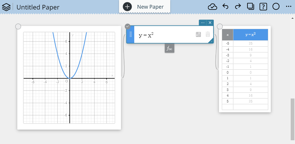
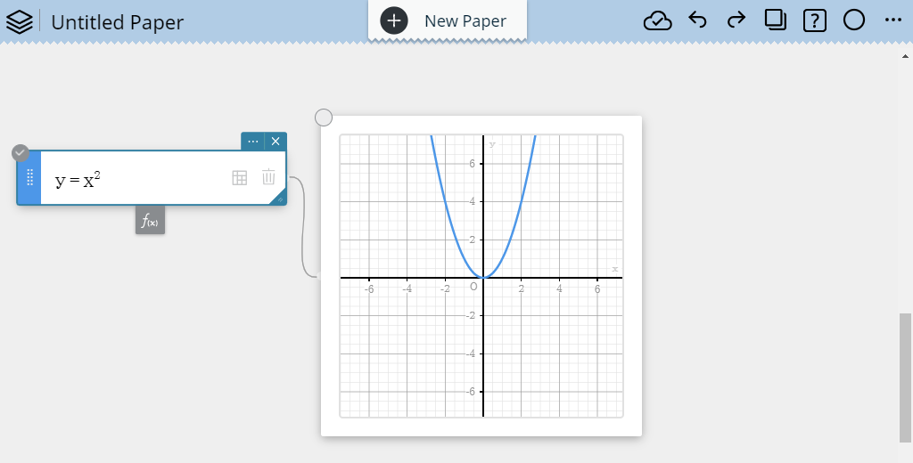
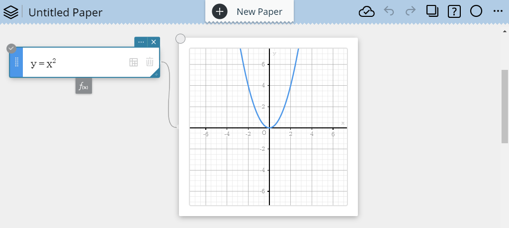
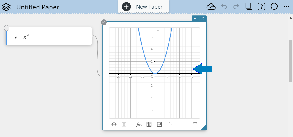
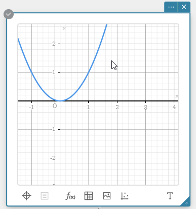
4. Use the soft keyboard to input a function. Example: $y = x^2$
5. On the soft keyboard, click [Execute].
• This draws the graph on the Graph Sticky Note.
6. On the Graph Function Sticky Note, click  .
.
• This displays a Table Sticky Note.
3-1-2. To input a numerical table and plot it on a graph
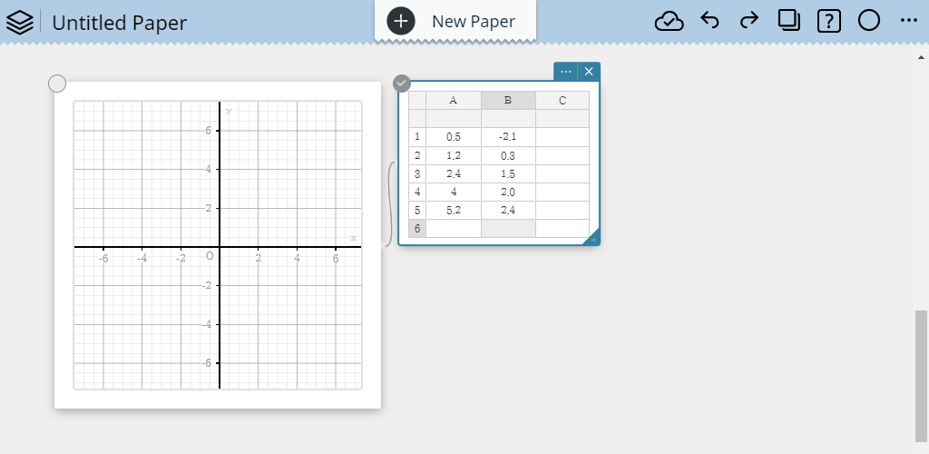
1. At the bottom of the Graph Sticky Note, click  to display a Statistical Data Sticky Note.
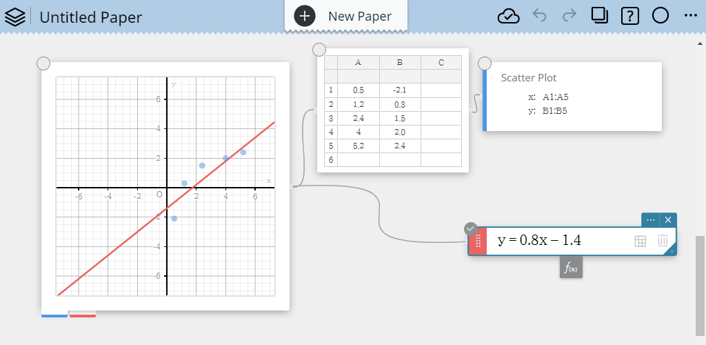
2. Input the data values you want to plot on the Statistical Data Sticky Note.
Example: Input the following for column A, rows 1 through 5: $0.5$、$1.2$、$2.4$、$4.0$、$5.2$ .
Input the following for column B rows 1 through 5: $-2.1$、$0.3$、$1.5$、$2.0$、$2.4$ .
• For information about how to input data values into a Statistical Data Sticky Note, see "4-1. Basic Statistical Calculation Operations".
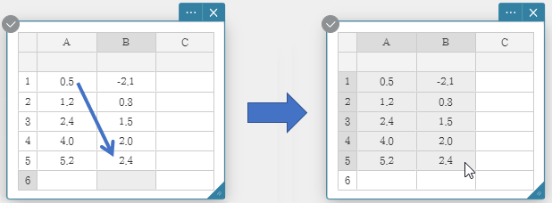
3. Drag from cell A1 to cell B5 (the range of data you want to plot).
• This selects the range of cells from cell A1 through cell B5.
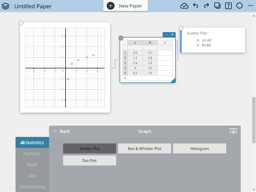
4. On the soft keyboard, click [Graph].
5. Click [Scatter Plot].
• This draws a scatter plot.
6. At the bottom of the Graph Sticky Note, click  .
.
• This displays a Graph Function Sticky Note.
7. Input the function: $y=0.8x-1.4$ on the Graph Function Sticky Note.
8. On the soft keyboard, click [Execute].
• This draws the graph.
3-2. Drawing Multiple Graphs
3-2-1. To graph multiple functions
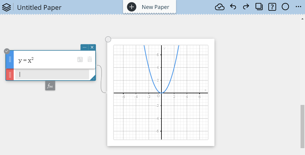
1. Click an existing Graph Function Sticky Note to select it.
2. At the bottom of the Graph Function Sticky Note, click  .
.
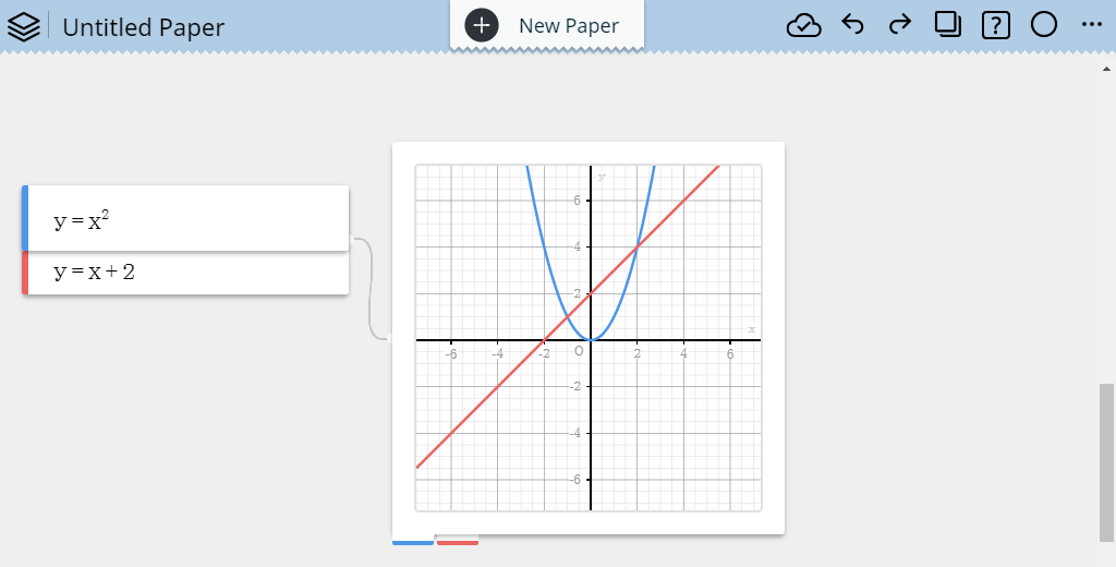
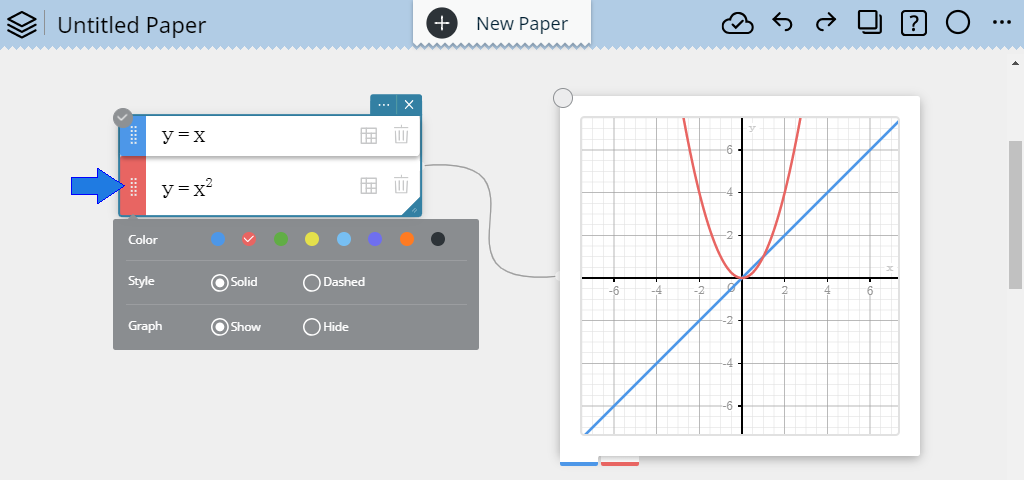
• This adds a new Graph Function Sticky Note.
3. Use the soft keyboard to input a function. Example: $y = x + 2$
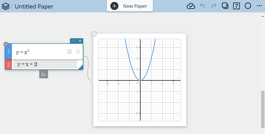
4. On the soft keyboard, click [Execute].
• This overwrites the existing graph with the new graph.
• You can overwrite up to 20 graphs by repeating steps 2 through 4 of this procedure.
3-2-2. To delete a particular function
1. Click the Graph Function Sticky Note to select it.
2. Click  on the Graph Function Sticky Note where the function you want to delete is input.
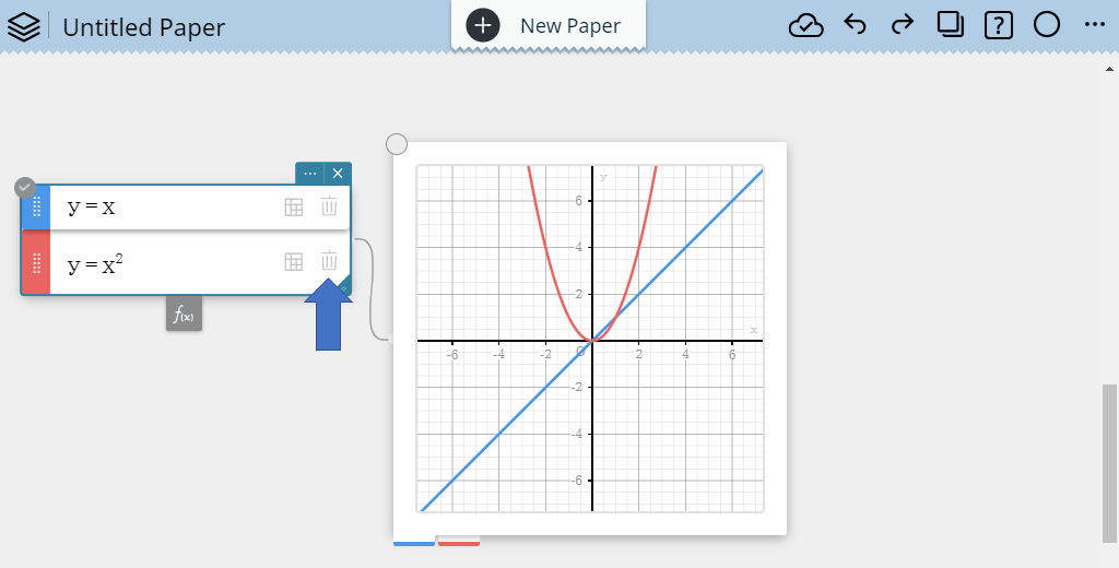
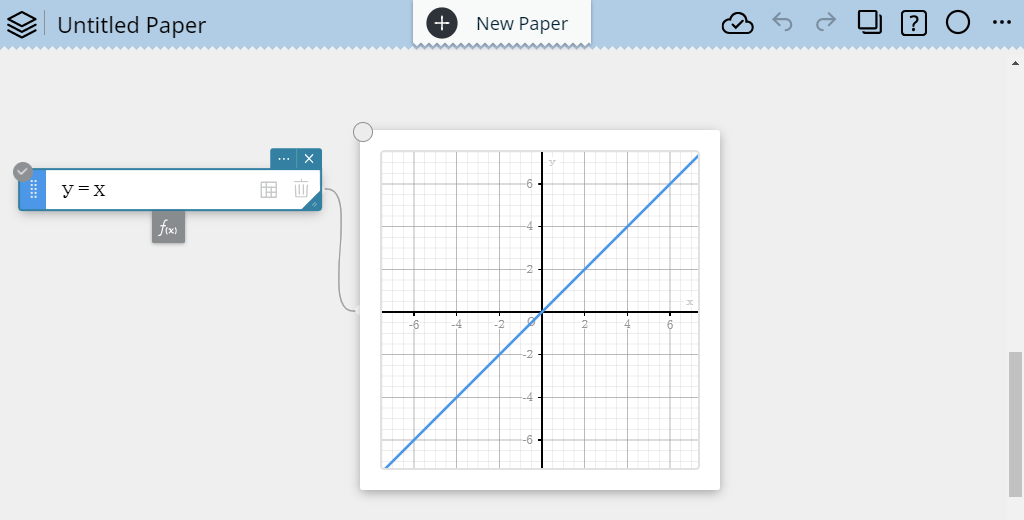
• This deletes the Graph Function Sticky Note, and also deletes the function and its corresponding graph.
Note
- If you just want to delete the function expression and graph without deleting the Graph Function Sticky Note, select the function expression input on the Graph Function Sticky Note and then press the [Delete] key.
3-3. Graphing a Rectangular Coordinate Equation($y=, x=$)
3-3-1. To graph a y= rectangular coordinate equation (y=)
1. At the bottom of the Graph Sticky Note, click  to create a Graph Function Sticky Note.
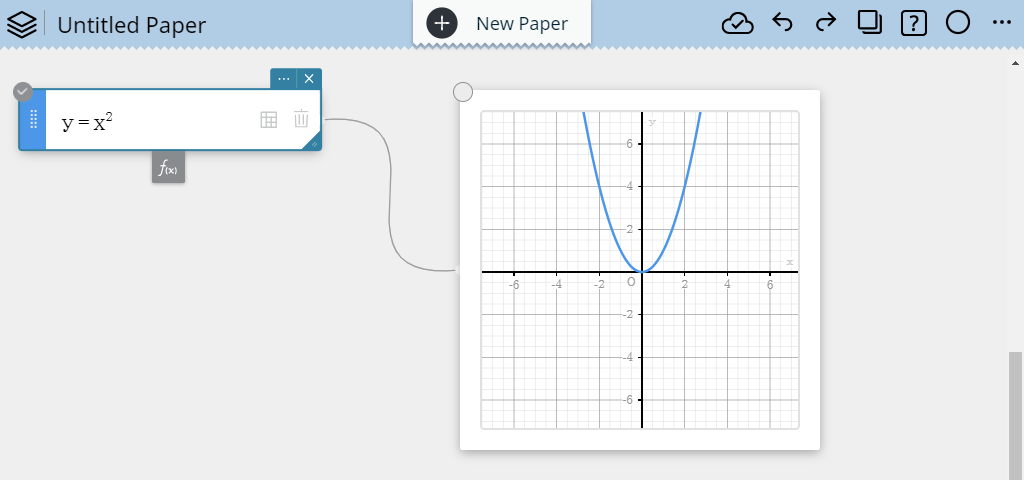
2. Use the soft keyboard to input the y= rectangular coordinate function (y=). Example:$y=x^2$
3. On the soft keyboard, click [Execute].
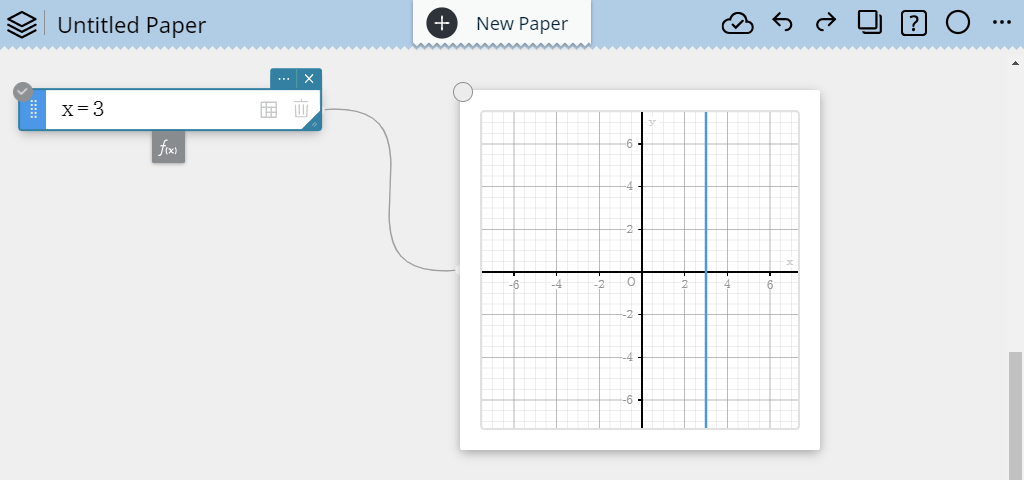
3-3-2. To graph a x= rectangular coordinate equation (x=)
1. At the bottom of the Graph Sticky Note, click  to create a Graph Function Sticky Note.
2. Use the soft keyboard to input the x= rectangular coordinate function. Example:$x=3$
3. On the soft keyboard, click [Execute].
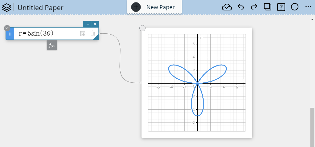
3-4. Graphing a Polar Coordinate Equation ($r=$)
1. At the bottom of the Graph Sticky Note, click  to create a Graph Function Sticky Note.
2. Use the soft keyboard to input the polar coordinate function.
Example: $r=5\sin(3\theta)$
3. On the soft keyboard, click [Execute].
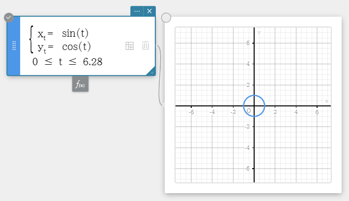
3-5. Graphing a Parametric Function
1. At the bottom of the Graph Sticky Note, click  to create a Graph Function Sticky Note.
2. On the soft keyboard, click  .
.
・This displays the input format for a parametric function.
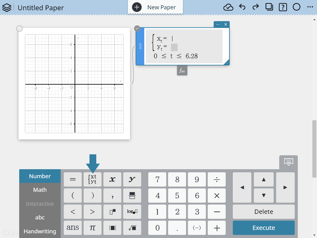
3. Input the parametric function.
Example: $x_{t}=\sin(t)$ $y_{t}=\cos(t)$
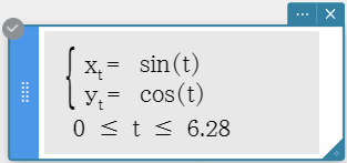
4. On the soft keyboard, click [Execute].
Note
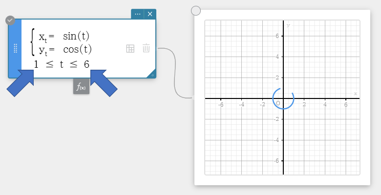
・You can change the range of t and draw the resulting graph.
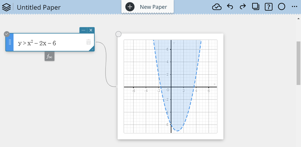
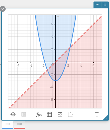
3-6. Graphing an Inequality
1. At the bottom of the Graph Sticky Note, click  to create a Graph Function Sticky Note.
2. Use the soft keyboard to input an inequality.
Example: $y>x^2-2x-6$
3. On the soft keyboard, click [Execute].
- Graphing is supported for inequalities expressed using the following forms:
$y \gt f(x)$
$y \lt f(x)$
$y \geq f(x)$
$y \leq f(x)$
Note
・< and > notation inequalities are graphed using a broken line. <= and >= notation inequalities are graphed using a solid line. A broken line means that values on the line are not included in the solutions, while a solid line means that values on the line are included in the solutions.
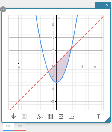
3-6-1. To specify the shading range
You can use this procedure to specify the shading range when simultaneously graphing multiple inequalities.
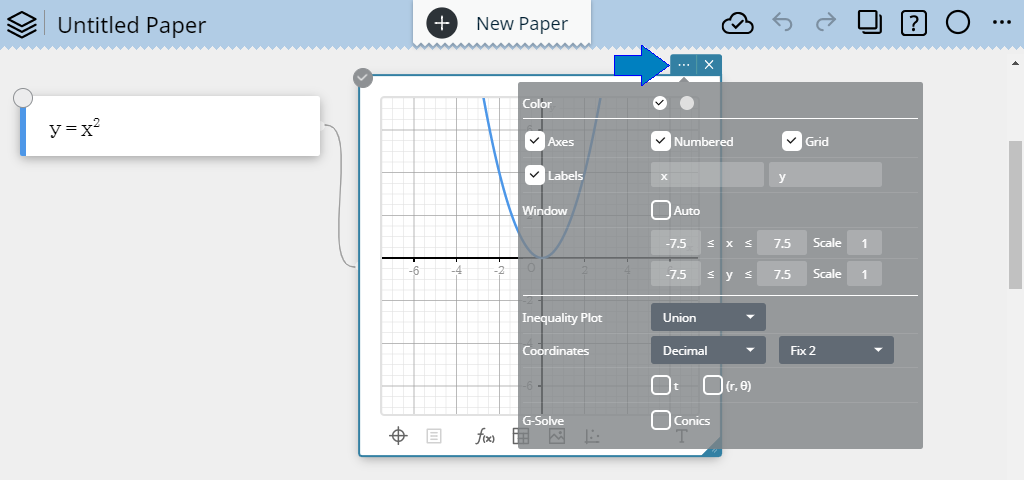
1. Click the Menu button ( ) of the Graph Sticky Note.
2. Use the Inequality Plot menu item to select [Union] or [Intersection].
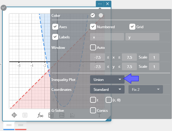
Union ... Shades all areas where the conditions of each of the graphed inequality are satisfied.
Intersection ... Shades only areas where the conditions of all of the graphed inequalities are satisfied.
Note
- If the conditions of an inequality are not satisfied and the Inequality Plot menu item setting is Union or Intersection, no shading is performed.
3-7. Drawing Circle, Elliptic, and Hyperbolic Graphs
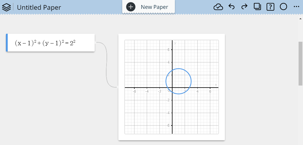
3-7-1. To draw a circle graph
1. At the bottom of the Graph Sticky Note, click  to create a Graph Function Sticky Note.
2. Use the soft keyboard to input a circle equation.
Example: $(x-1)^2+(y-1)^2=2^2$
3. On the soft keyboard, click [Execute].
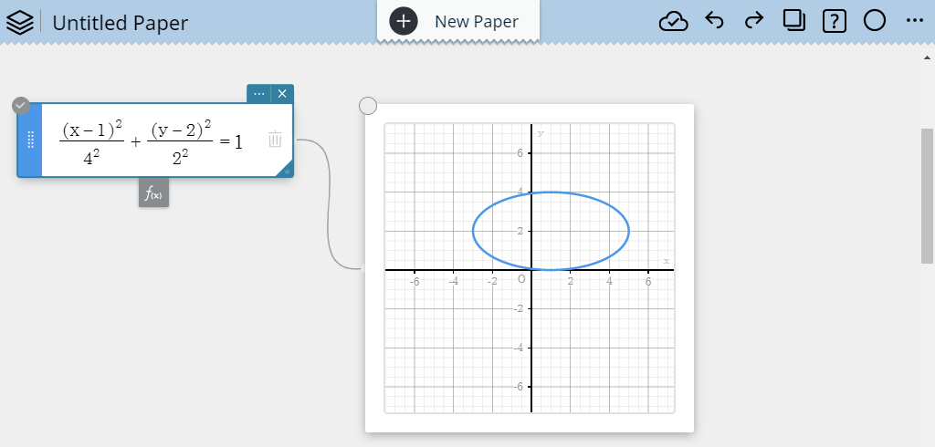
3-7-2. To draw an elliptic graph
1. At the bottom of the Graph Sticky Note, click  to create a Graph Function Sticky Note.
2. Use the soft keyboard to input an elliptic equation.
Example:
$$ \cfrac{(x-1)^2}{4^2}+\cfrac{(y-2)^2}{2^2}=1 $$
3. On the soft keyboard, click [Execute].
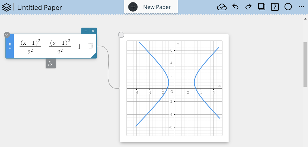
3-7-3. To draw a hyperbolic graph
1. At the bottom of the Graph Sticky Note, click  to create a Graph Function Sticky Note.
2. Use the soft keyboard to input a hyperbolic equation.
Example:
$$ \frac{(x-1)^2}{2^2}-\frac{(y-1)^2}{2^2}=1 $$
3. On the soft keyboard, click [Execute].
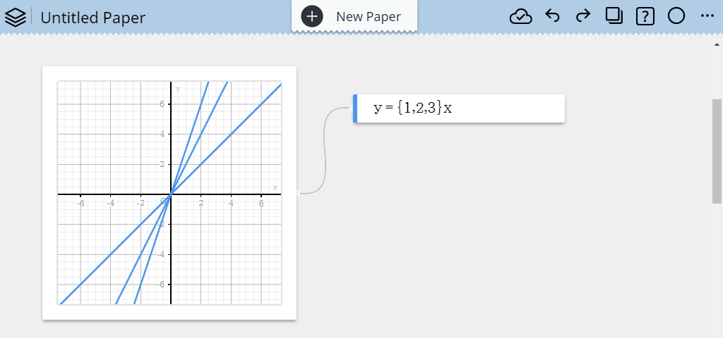
3-8. Using a List of Values to Draw Multiple Graphs
You can use a list as a coefficient in a function and simultaneously draw multiple graphs.
1. At the bottom of the Graph Sticky Note, click  to create a Graph Function Sticky Note.
2. Input a function expression with a form that includes a list in a coefficient.
Example: $y=${$1,2,3$}$x$
3. On the soft keyboard, click [Execute].
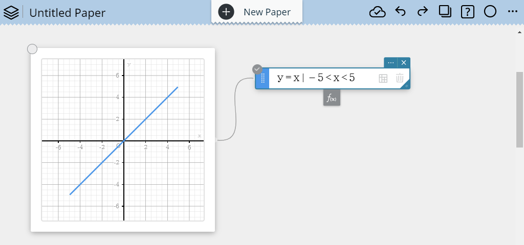
3-9. Specifying a Range to Draw a Graph
You can specify a range for drawing a graph.
To do so, input a function using the syntax below.
<function>|<inequality specifying draw range>
1. At the bottom of the Graph Sticky Note, click  to create a Graph Function Sticky Note.
2. Input a function expression with a draw range specification.
Example: $y=x|-5<x<5$
3. On the soft keyboard, click [Execute].
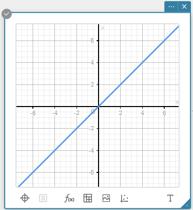
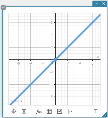
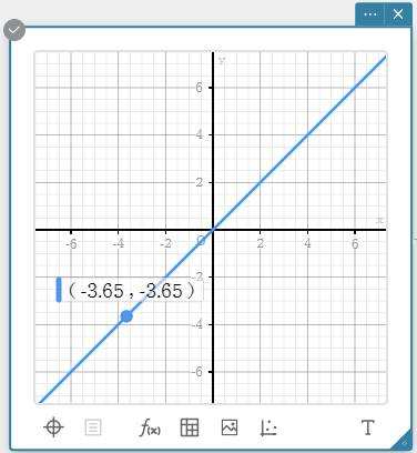
3-10. Using Trace
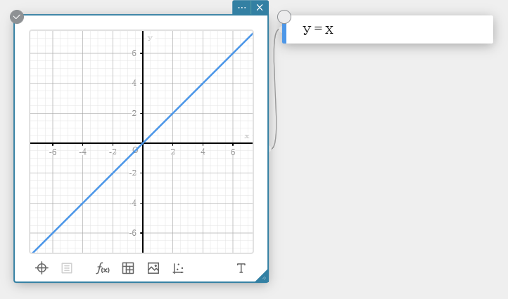
With trace, you can click a graph line to plot a point on it and display the coordinates at that point. You can also drag the point along the graph line.
1. Draw a graph.
Example: $y=x$
2. Click the Graph Sticky Note to select it.
3. Click the graph to select it.
・This causes the line of the selected graph to become thicker.
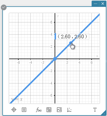
4. Click the graph line.
• This plots a point on it, and display the corresponding coordinates.
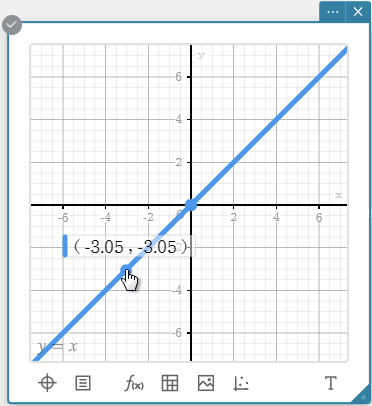
5. Drag the point along the graph line.
• You can move the point along the graph.
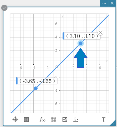
Note
- You can also plot multiple points on the graph line.
3-10-1. To delete a point plotted on a graph line
1. Click the point you want to delete.
・This displays  in the upper right corner of the point coordinate display box.
2. Click the "×" .
• This deletes the point.
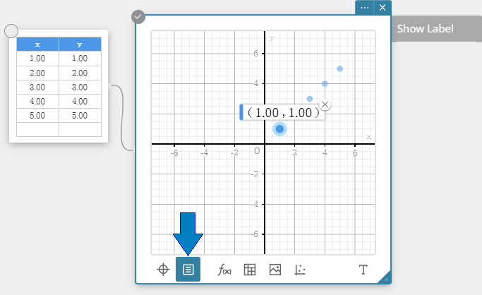
3-10-2. To use coordinate values in a calculation
1. Draw a graph.
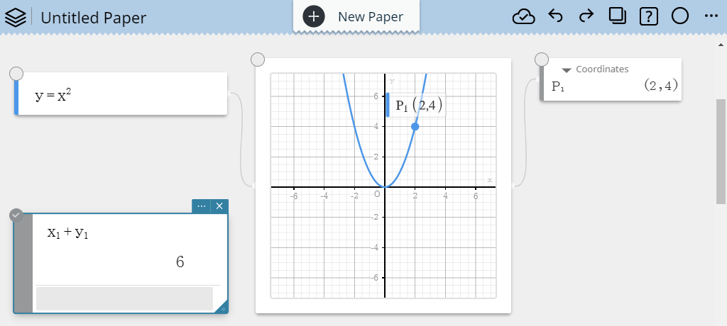
Example: $y=x^2$
2. Click the graph line to plot a point on it.
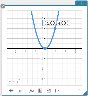
3. Click the point again to select it.
4. At the bottom of the Graph Sticky Note, click 
• This displays the Property menu.
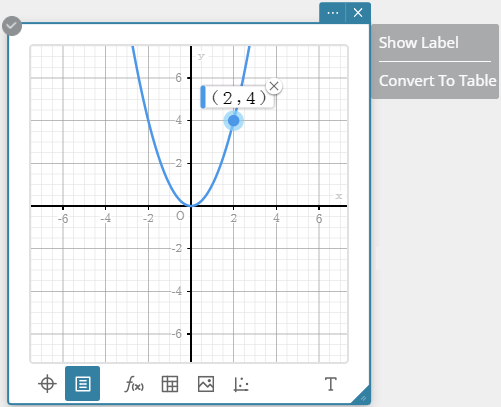
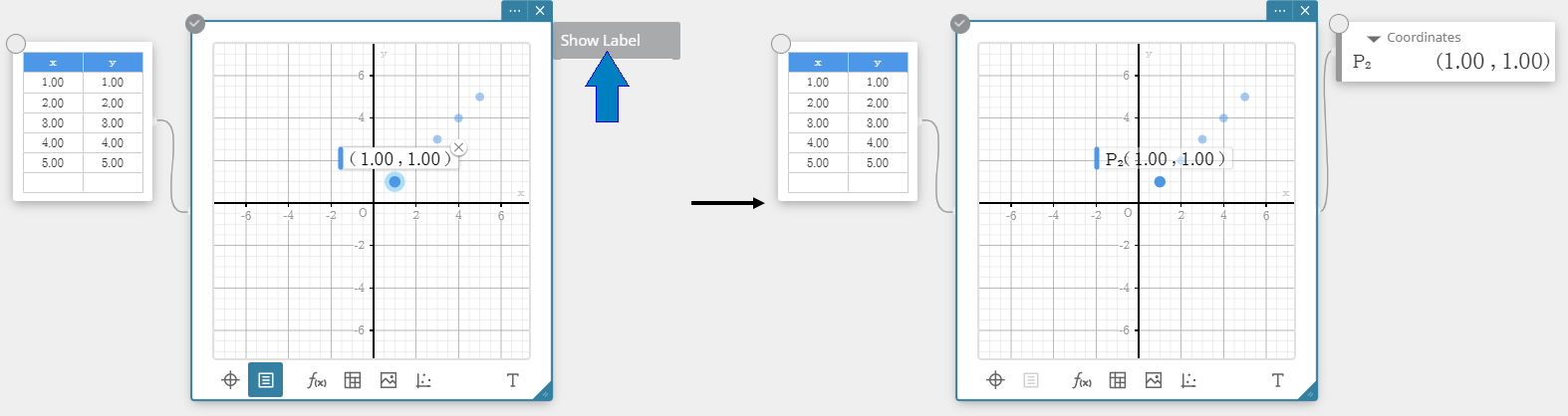
5. Click [Show Label].
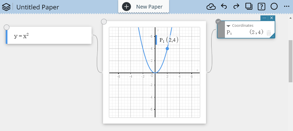
• This creates a Coordinates Sticky Note.
6. Create a Calculate Sticky Note.
7. On the Calculate Sticky Note, input the expression using the coordinates: $x_{1}+y_{1}$ .
8. On the soft keyboard, click [Execute].
• This displays the expression's calculation result using the coordinate values.
Note
- You can repeat steps 2 and 5 above and create multiple Coordinates Sticky Notes, if you like.
- Instead of clicking in step 4, you can also right-click a plotted point to display the Property menu.
- Creating a Coordinate Sticky Note adds a ${\rm P}_n$ ($n$ = serial number) label to the corresponding point. The ${\rm P}_n$ x-coordinate value is stored to variable $x_n$, and the y-coordinate value is stored to variable $y_n$.
- Deleting a Coordinate Sticky Note also deletes the corresponding points.
3-11. Basic Graph Analysis Operations
Clicking on a graph you have drawn will automatically perform appropriate analysis (for example: roots, maximum value, minimum value, directrix, axis of symmetry) depending on the graph type.
1. Draw a graph.
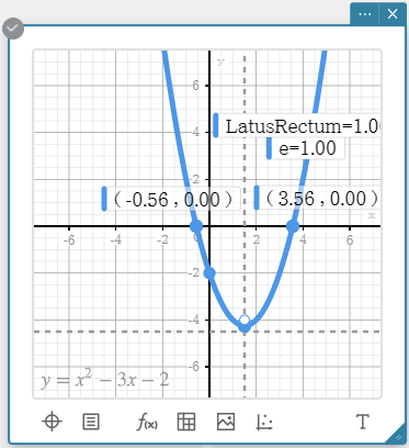
Example: $y=x^2-3x-2$
2. Click the Graph Sticky Note to select it.
3. Click the Menu button ( ).
).
4. Select the [Conics] check box.
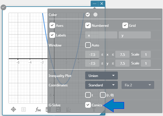
・This enables graph analysis that is characteristic of conics (directrix, axis of symmetry, focus, etc.)
5. Click the Graph Sticky Note, and then click the graph.
・This analyzes the graph and displays dots (●) at the analysis result coordinate points.
・The directrix and axis of symmetry are shown as broken grey lines.
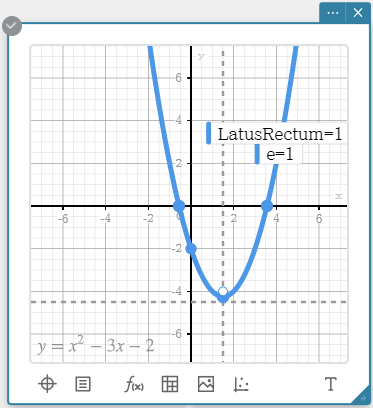
6. Click a dot (●).
• This displays its coordinates.
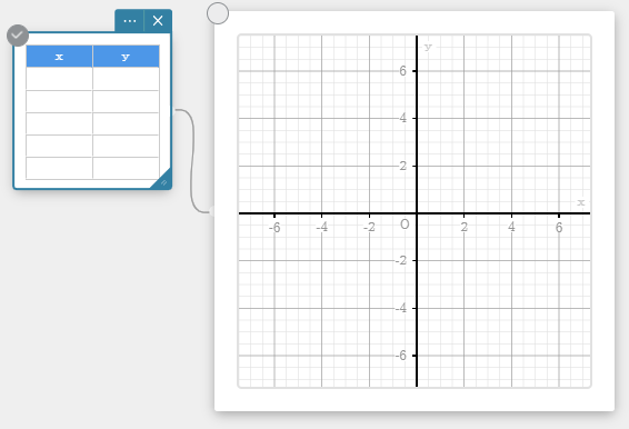
3-12. Creating a Table
3-12-1. To create a table from a function
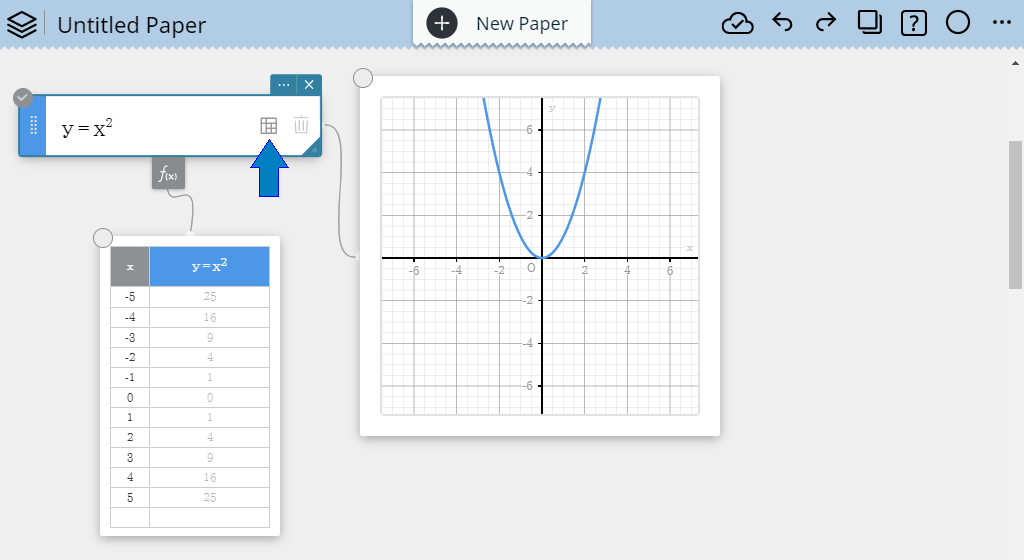
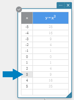
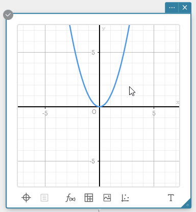
1. Draw a graph. Example: $y=x^2$
2. On the Graph Function Sticky Note, click  .
.
• This creates a Table Sticky Note. The table generated from the function will appear in the Table Sticky Note.
3-12-2. To create a table by plotting points on a graph
1. Draw a graph. Example: $y=x^2$

2. Click the Graph Sticky Note to select it.
3. Sequentially click different locations on the graph to plot multiple points.
4. Sequentially click the plotted points to select them.
5. At the bottom of the Graph Sticky Note, click  .
.
• This displays the Property menu.
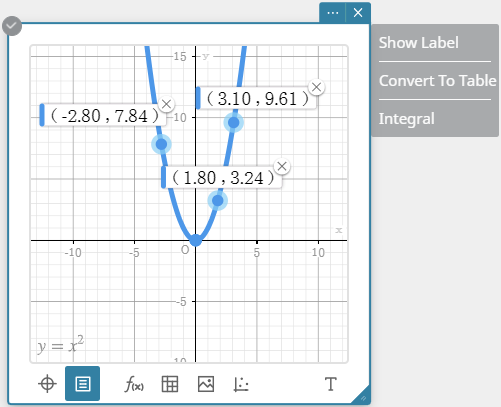
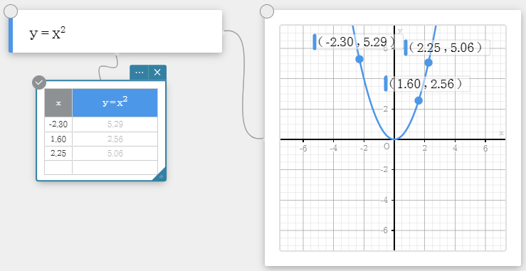
6. Click [Convert To Table].
• This displays a Table Sticky Note. The coordinate values of the plotted points you selected in step 4 above will be input on the Table Sticky Note.
Note
- Instead of clicking in step 5, you can also right-click a plotted point to display the Property menu.
3-13. Editing a Table
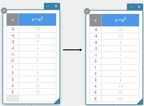
3-13-1. To add a row to a table
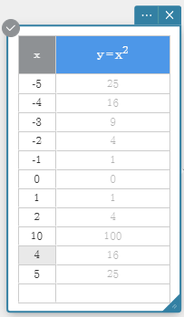
1. Click the Table Sticky Note.
2. Input a value into the bottom-most cell of the independent variable column (lower left cell).
• This adds a row at the bottom of the table.
3. On the soft keyboard, click [Execute].
3-13-2. To delete a row from a table
1. Click the Table Sticky Note.
2. Right-click the cell of the independent variable column whose row you want to delete.
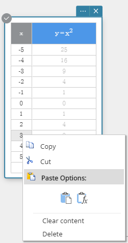
3. Click [Delete].
• This deletes the row.
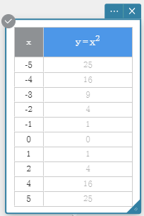
3-13-3. To change a value in a table
1. On the Table Sticky Note, click the value you want to change.
2. Input the new value.
3. On the soft keyboard, click [Execute].
3-14. Using a Slider
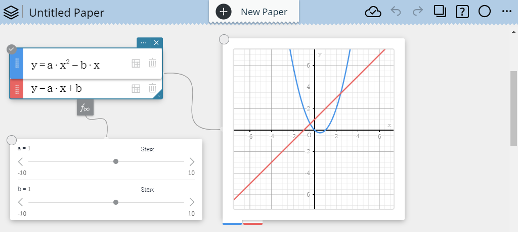
You can change the value of a variable in a graph expression (for example, the value of a in $y=a \cdot x^2$) from the graph screen and observe how the change affects the graph.
1. Input a function that includes variables into a Graph Function Sticky Note. This will display sliders for changing the values assigned to the variables.
Example: $y= a \cdot x^2-b \cdot x \hspace{10mm} y=a \cdot x+b$
• This will display sliders for changing the values assigned to the variables.
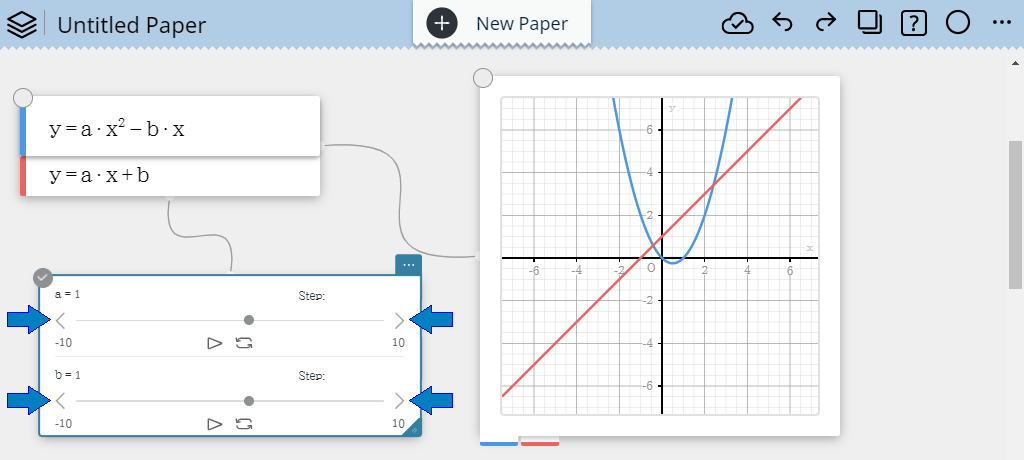
2. Click one of the arrow buttons (< or >) on either end of the slider.
・This will change the corresponding value and re-draw the graph accordingly.
Note
- You can use a slider to change the value (variable value, lower limit value, upper limit value, step value) displayed above the slider. Click the value you want to change.
- Clicking the arrow (
 ) below a slider starts automatic change of the variable value and re-drawing of the graph with the new values (animation). To stop the animation, click
  .
.  and
and  indicate the animation playback style.
  indicates that playback will go left to right, and then repeat left to right.
  indicates that playback will go left to right, and the right to left. Click
  or
or  to toggle between playback types.
3-15. Configuring Graph Display Settings
1. Click the Graph Sticky Note.
2. Click the Menu button ( ).
).
3. Configure display settings and adjust the display range.
-
Axes: Select this check box to show the coordinate axes in the draw area. Numbered: Select this check box to show the tick marks in the draw area. To be able to select this check box, you first need to select the" Axes" check box. Grid: Select this check box to show a grid in the draw area. Labels: Select this check box to show coordinate axis names on the graph.
You can change an axis name, if you want.Window: Select this check box to specify a display range that is optimized for statistical data. Stat-Auto: Selecting this check box automatically optimizes the graph display range and draws the graph. π: Selecting this check box changes the scale of the x-axis scale to π. 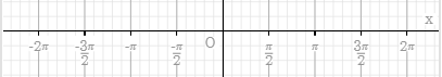
X: Specifies the display range of the x-axis. X Scale: Specifies interval between tick marks on the x-axis. If the π check box is selected, clicking this field displays a menu that can be used to change the display range setting. Y: Specifies the display range of the y-axis. Y Scale: Specifies interval between tick marks on the y-axis. Inequality Plot: Use this setting to specify the shading range when simultaneously graphing multiple inequalities. Intersection: Shades only areas where the conditions of all of the graphed inequalities are satisfied. Union: Shades all areas where the conditions of each of the graphed inequality are satisfied. Coordinates: Configures the coordinate value display setting. Decimal: Displays coordinate values using decimal fractions. Standard: Displays coordinate values using expressions. t: Select this check box to display parametric graph coordinate values as t values. ($r$, $\theta$): Select this check box to display polar graph coordinate values as $r$ and $\theta$ values. Conics: Select this check box to display analysis results that are characteristic of conics (directrix, axis of symmetry, focus, etc.)
3-16. Zooming a Graph
3-16-1. To zoom a graph
1. Click the Graph Sticky Note.
2. Move the mouse pointer to the location you want to zoom.
3. Rotate the scroll wheel of your mouse to zoom the graph.
Note
- If you are using a smartphone or tablet, you can zoom by pinching in or pinching out.
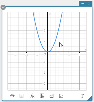
- To return to the default display, click
 in the lower-left corner of the Graph Sticky Note. On the menu that appears, select [Default Zoom]
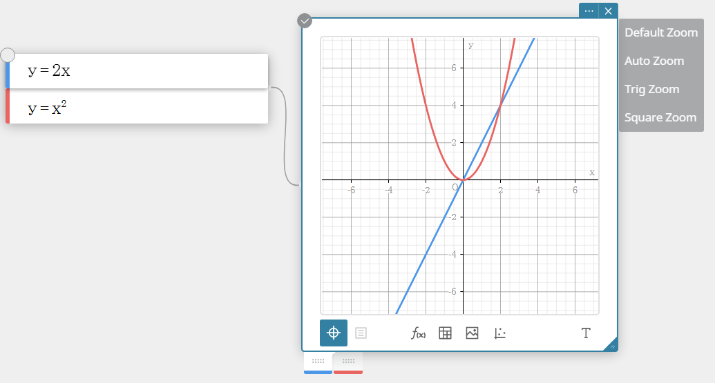
3-16-2. To configure the graph display range setting (Zoom Options)
1. Click a Graph Sticky Note.
2. In the lower-left corner of the Graph Sticky note, click .
・This displays a zoom options menu to the right of the Graph Sticky Note.
-
Default Zoom: Initial default display zoom according to the size of the Graph Sticky Note. Auto Zoom: Automatically sets the range so the features* of the graph fit within the drawing range.
* For example, the x- or y-axis intersect, the intersection of two graphs, the inflection point, limits, etc.Trig Zoom: Sets a new scale according to the current angle unit setting (degrees, radians, grads). Square Zoom: Automatically corrects the value on the y-axis side so the x-axis and y-axis scales have a ratio of 1: 1.
3. Select the zoom option you want from the menu.
・The graph display range and x-axis and y-axis scales are set automatically according to the zoom option you select.
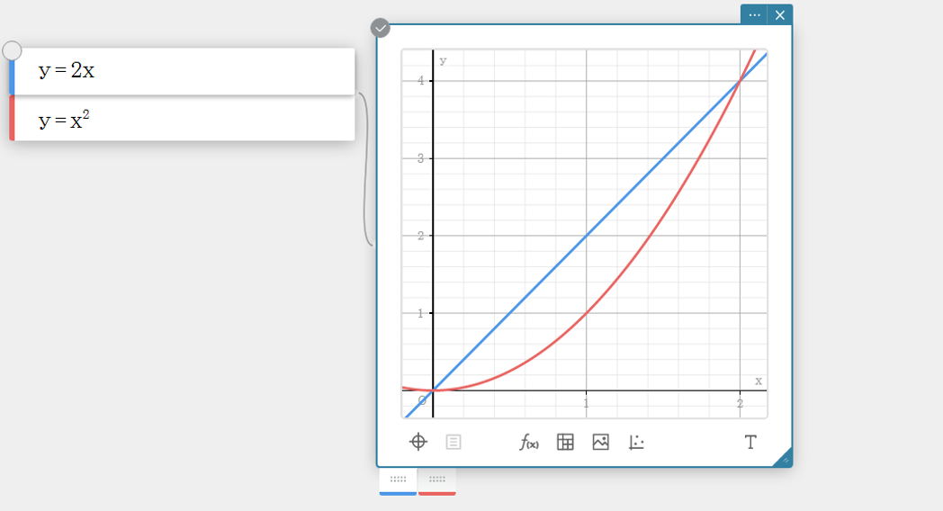
Example display when "Auto Zoom" is selected
3-17. Panning a Graph
1. Click the Graph Sticky Note.
2. Move the mouse pointer to the location you want to pan.
3. Drag the graph to pan it.
Note
-
To return to the default display, click
 in the lower-left corner of the Graph Sticky Note. On the menu that appears, select [Default Zoom].
3-18. Changing the color of a Graph
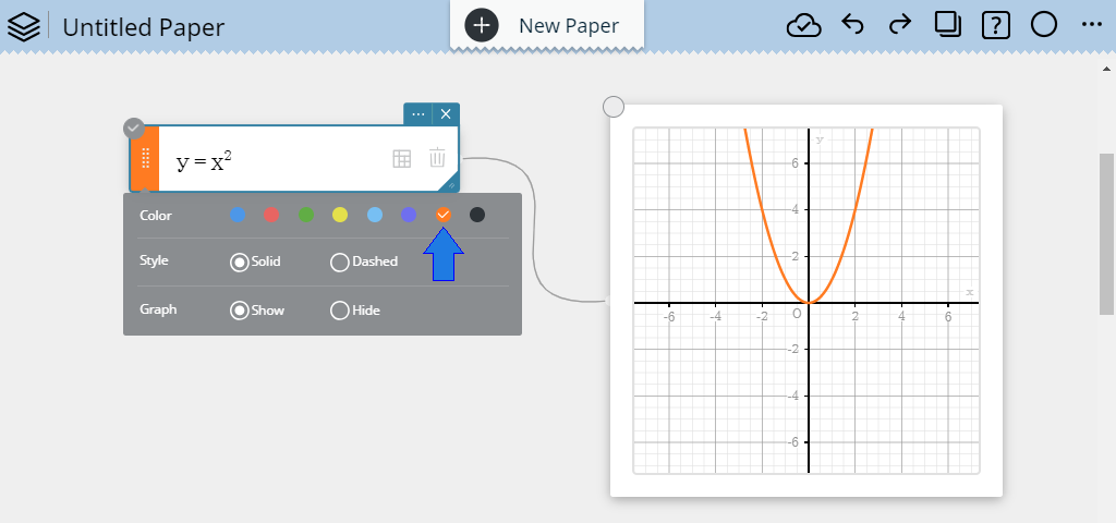
1. Click the drag handle ( ) of the Graph Function Sticky Note.
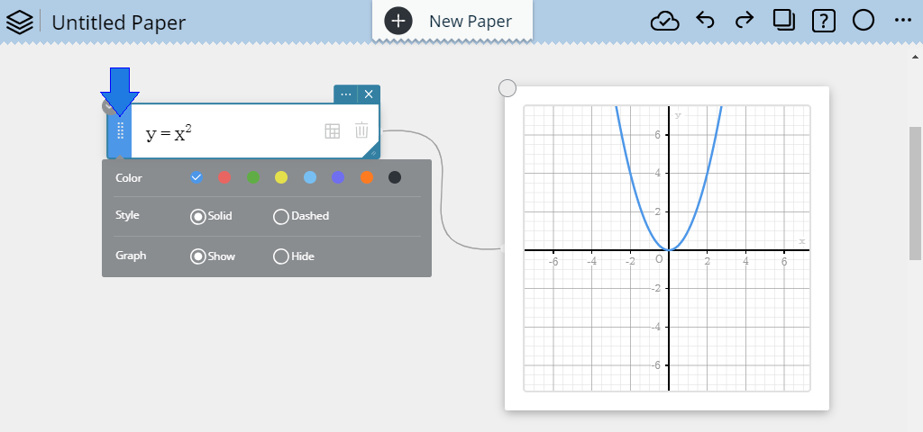
2. On the Color Palette, select the desired color.
• This changes the graph color.
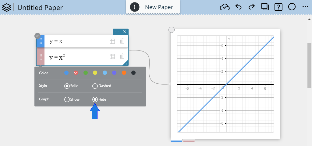
3-19. Hiding a Graph
1. Draw a graph.
2. Click the drag handle ( ) of the Graph Function Sticky Note.
3. Click [Hide].
・This hides the graph of the selected function.
Note
- To re-display the graph, click [Show] in step 3 above.
3-20. Displaying a Background Image
1. At the bottom of the Graph Sticky Note, click  .
.
・This creates an Image Sticky Note.
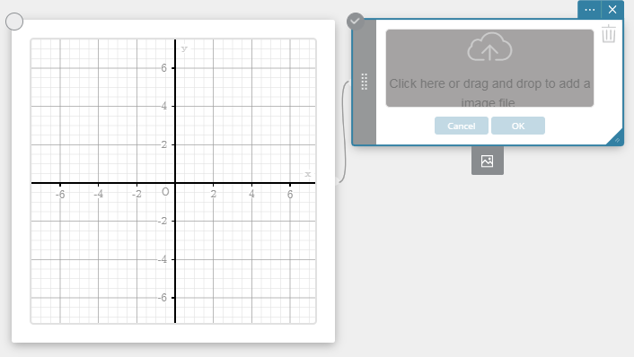
2. Click  .
.
・This displays a dialog box for opening a file.
3. Select the image file you want and then click [Open].
4. On the Image Sticky Note, click [OK].
・This displays the image selected with the Graph Sticky Note.
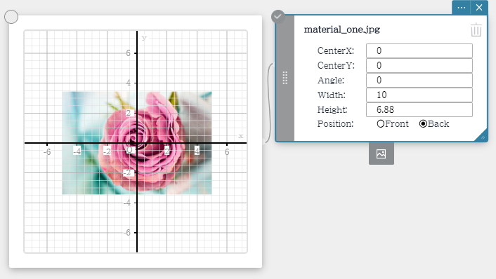
・You can configure the settings below for an Image Sticky Note.
- CenterX: Specifies the x-axis value of the image center.
- CenterY: Specifies the y-axis value of the image center.
- Angle: Specifies the image rotation angle.
- Width: Specifies the image width.
- Height: Specifies the image height.
-
Position:
- Front・・・Displays the image in front of the coordinate axes and the grid.
- Back・・・Displays the image in back of the coordinate axes and the grid.
Note
・Instead of performing steps 2 and 3, you can also drop the desired image file onto the Image Sticky Note.
・You can create multiple Image Sticky Notes by clicking the Image Sticky Note's  . You can also display multiple images by repeating steps 1 through 4 for the newly created Image Sticky Note.
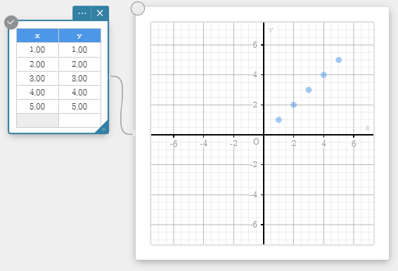
3-21. Plot Function
3-21-1. To plot points on a graph
1. At the bottom of the Graph Sticky Note, click  .
.
・This creates a Plot Sticky Note.
2. On the Plot Sticky Note, input the x-coordinate and y-coordinate values of the points you want to plot.
・This plots points at the coordinates you input.
Note
・You can configure the settings shown below by clicking  on a Dot Plots Sticky Note.
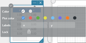
- Plot color: Specifies the color of the plotted points.
- Labels: Specifies the label names.
- Lock: Locks selected cell(s). If the selected cells are locked, this item unlocks the cells.
3-21-2. To display the Coordinates Sticky Note of a point
1. Click a plotted point.
・This displays the coordinates of the Point.
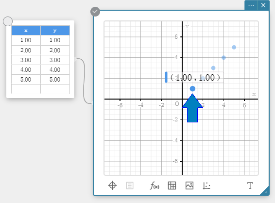
2. Click the displayed coordinate values.
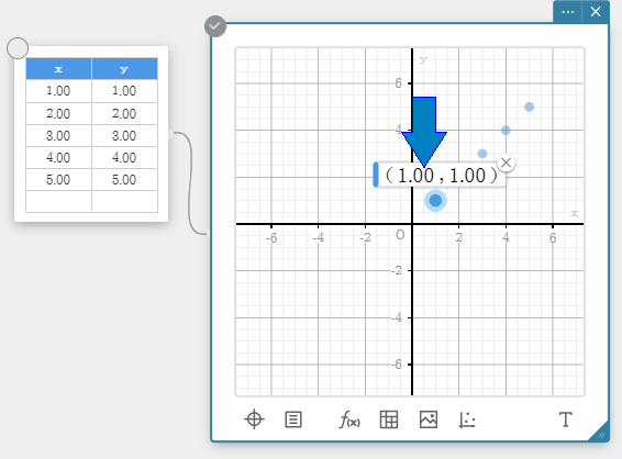
3. Click  .
.
• This displays the Property menu.
4. Click [Show Label].
• This displays a Coordinates Sticky Note.
Note
- Instead of clicking in step 3, you can also right-click a displayed coordinate to display the Property menu.
3-22. Inputting Text
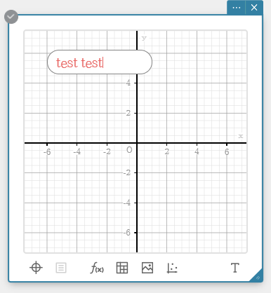
1. At the bottom of the Graph Sticky Note, click  .
.
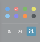
• This enables text input and displays the text palette.
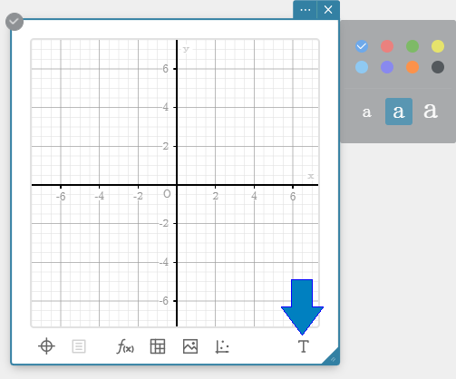
2. Use the text palette to specify the text color and size.
3. Click the location where you want to input text.
4. Input a text string.
Note
-
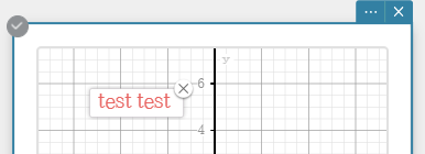
Clicking input text selects it. You can perform the operations below on selected text.
• You can reposition text by dragging it.
• Clicking
 will display the text palette, which can be used to change the color and size of the text.
• To delete text, click
 .
. - Double-clicking input text selects it for editing.
3-23. Determining the Integral Value and Area of a Region
1. Draw a graph.
2. Select the graph and then click  .
.
3. Click "Integral".
・This displays an Integral/Area Sticky Note.
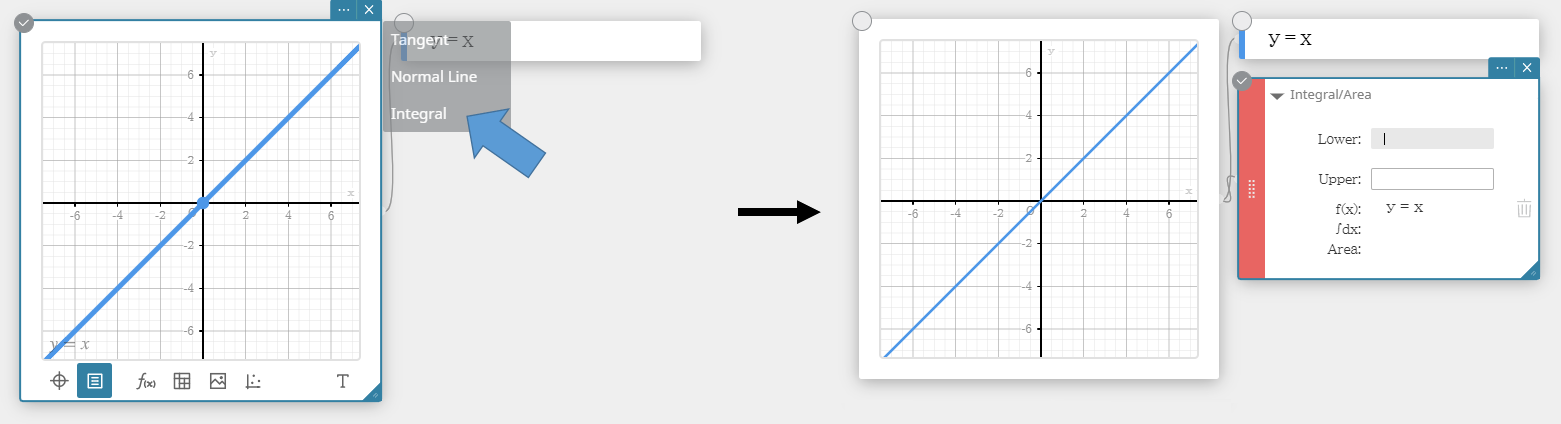
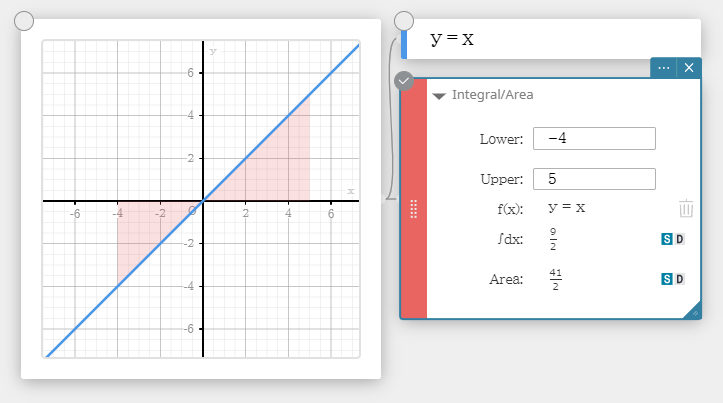
4. Input the lower limit value and upper limit value of the integration.
5. On the soft keyboard, click [Execute].
・This calculates the integral and area, and shades the integration.
3-24. Drawing a Line Tangent or Normal to a Graph
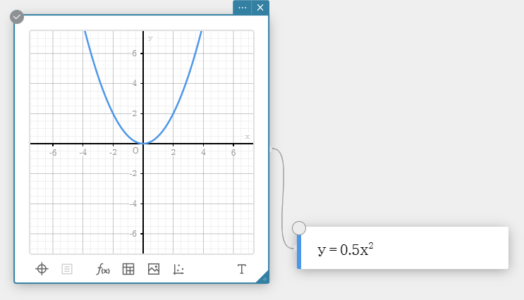
3-24-1. To draw a line tangent to a graph
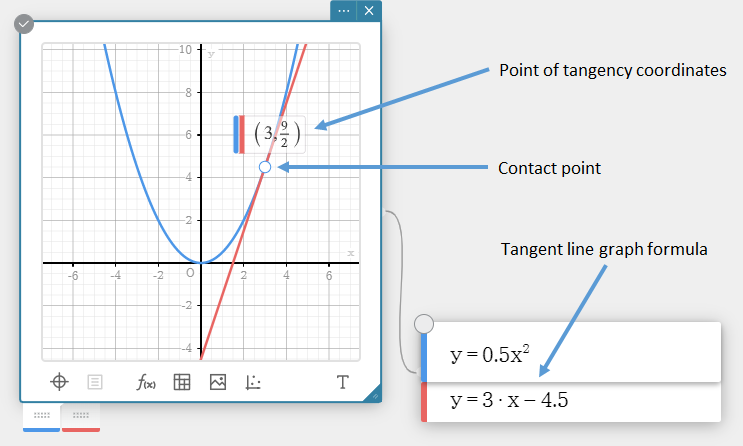
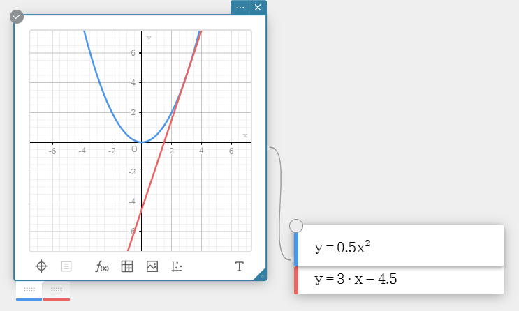
Example: To draw a line that is tangent to graph $y=0.5x^2$
1. Graph $y=0.5x^2$
2. Click the Graph Sticky Note to select it.
3. Click any point on the graph.
• This selects the graph and causes the line of the graph to become thicker.
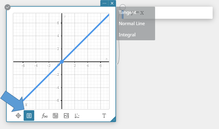
4. Click  .
.
5. Click "Tangent".
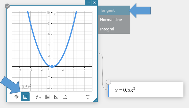
• This will draw a line tangent to graph $y=0.5x^2$, and creates a Graph Function Sticky Note that corresponds to the tangent simultaneously.
• The coordinates of the point of tangency (contact point) will be indicated by  .
.
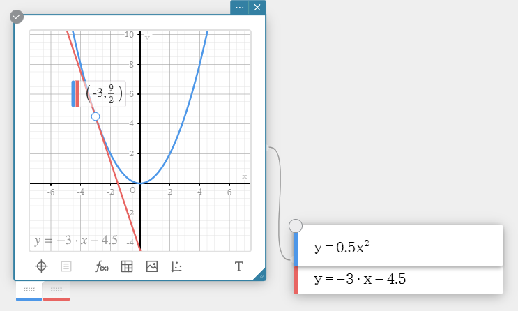
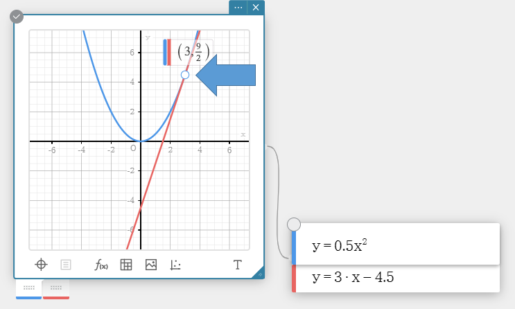
6. Drag the contact point ( ).
).
• You can reposition the location of the point of tangency.
Note
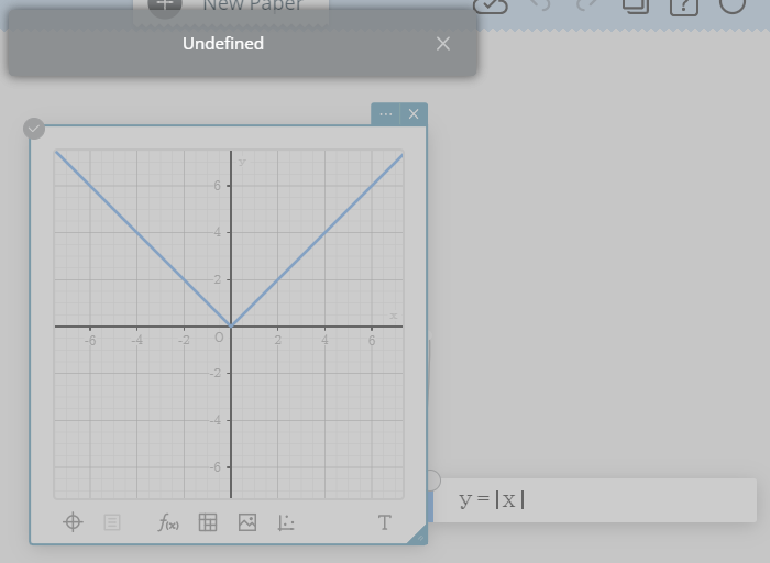
- If you specify coordinates on a graph for which a tangent line cannot be defined, a not-defined error occurs. If a not-defined error occurs, the tangent and the tangent graph expression are deleted from the Sticky Note.
Example: When coordinates $(0, 0)$ is specified on the graph "$y={\rm abs}(x)$".
3-24-2. To draw a line that is normal to a graph
Perform the same steps as those under "3-24-1. To draw a line tangent to a graph", except as noted below.
- In step 3, click "Normal Line" instead of "Tangent".
3-24-3. To delete a contact point
1. Click the contact point to select it.
• This displays  in the upper right corner of the contact point coordinate display box.
2. Click .
• This will delete the contact point. At this time the tangent line and its Graph Sticky Note will remain on the display, but without a contact point.
3-25. Graph Analysis Functions
| Trace | |
|---|---|
| Plots a point on the currently select graph and displays its coordinates. You can also drag the point along the graph line. | 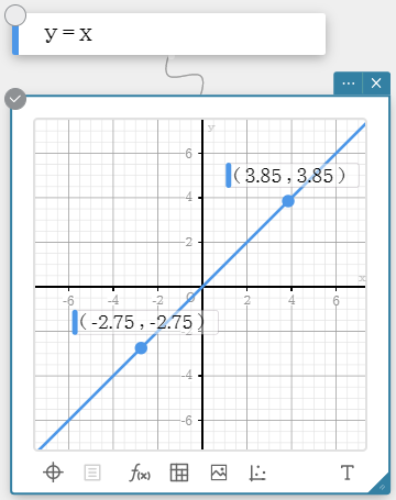 |
| x-Intercept | |
| Displays the point where the graph intercepts the X-axis (x-Intercept). Click a point to show its coordinates. | 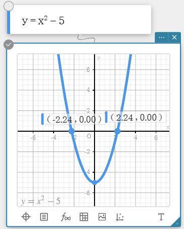 |
| Min | |
| Displays a point at the minimum value of a graph. Click the point to show its coordinates. | 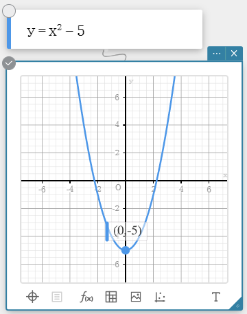 |
| Max | |
| Displays a point at the maximum value of a graph. Click the point to show its coordinates. | 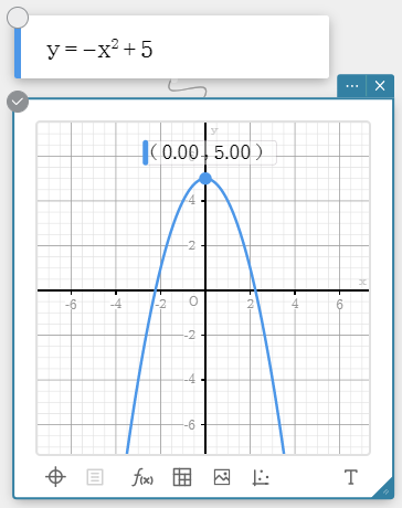 |
| y-Intercept | |
| Displays the point where the graph intercepts the Y-axis (y-Intercept). Click a point to show its coordinates. |  |
| Intersection | |
| Displays the points of intersection of two graphs and displays them. Click a point to show its coordinates. | 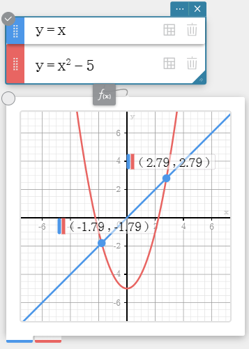 |
| Focus | |
| Displays the focus of a parabolic graph, elliptic graph, or hyperbolic curve graph. Click the point to show its coordinates. | 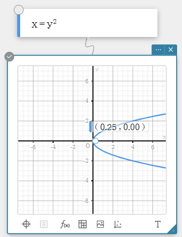 |
| Vertex | |
| Displays the vertex of a parabolic graph, elliptic graph, or hyperbolic curve graph. Click a point to show its coordinates. | 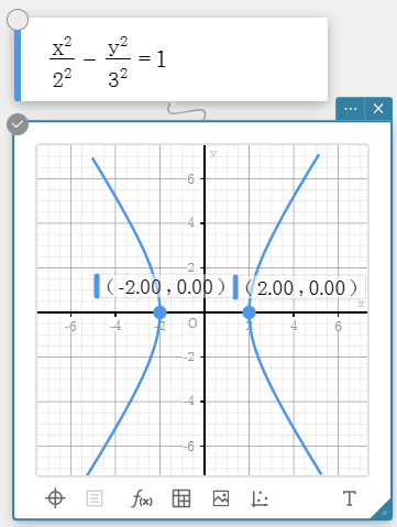 |
| Directrix | |
| Displays the directrix of a parabolic graph. Clicking a directrix displays the directrix expression (x=, y=). | 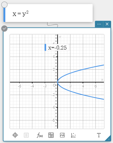 |
| Symmetry | |
| Displays the axis of symmetry of a parabolic graph. Clicking the axis of symmetry displays the axis of symmetry expression (x=, y=). | 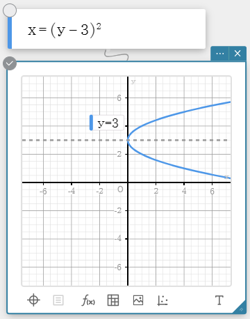 |
| Latus Rectum Length | |
| Displays the length of the latus rectum of a parabolic graph. (The value is displayed after "LatusRectum=".) | 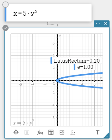 |
| Center | |
| Displays the center of a circle graph, elliptic graph, or hyperbolic curve graph. Click the point to show its coordinates. | 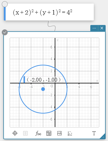 |
| Radius | |
| Displays the radius of a circle graph. Click the radius to show its length ($r=$). | 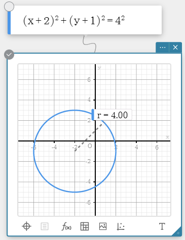 |
| Asympotes | |
| Displays the asympotes of a hyperbolic curve graph. Click an asympote to show its equation. | 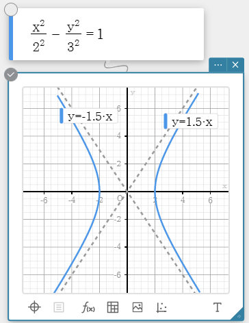 |
| Eccentricity | |
| Displays the eccentricity of a parabolic graph, elliptic graph, or hyperbolic curve graph. (The value is displayed after ($e=$).) | 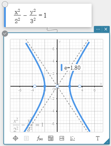 |