Advanced

solve

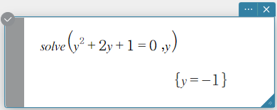
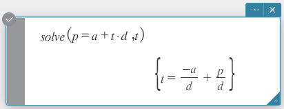
Returns the solution of an equation or inequality.
Syntax 1: solve(Exp/Eq/Ineq [, Variable] [ ) ]

• “\(x\)” is the default when you omit “[, Variable]”.

Syntax 2: solve(Exp/Eq/Ineq\(≠\), Variable[, value, lower limit, upper limit] [ ) ]

• This command is valid only for equations and \(≠\) expressions when “value” and the items following it are included. In that case, this command returns an approximate value.
• A true value is returned when you omit “value” and the items following it. However, when a true value cannot be obtained, an approximate value is returned for equations only based on the assumption that value = 0, lower limit = – ∞, and upper limit = ∞.

Syntax 3: solve({Exp-1/Eq-1, …, Exp-N/Eq-N}, {Variable-1, …, Variable-N} [ ) ]

• When “Exp” is the first argument, the equation Exp = 0 is presumed.

Syntax 4:
Entering a vector equation in the solve( command allows the relationship between 2 objects (points, lines, planes or spheres) to be resolved. Here, 4 typical examples of syntax are shown for solving a vector equation using the solve( command.

The syntax below shows a column vector with 3 (or 2) elements between Vct-1 and Vct-6), with s, t, u and v as the parameters.
solve(Vct-1 + s * Vct-2 [= Vct-3, {variable-1}])

• If the right side of the equation (= Vct-3) is omitted in the above syntax, it is assumed that all of the elements on the right side are 0 vectors.
  solve(Vct-1 + s * Vct-2 = Vct-3 + t * Vct-4, {variable-1, variable-2})
  solve(Vct-1 + s * Vct-2 + t * Vct-3 = Vct-4 – u * Vct-5, {variable-1, variable-2, variable-3})
  solve(Vct-1 + s* Vct-2 + t * Vct-3 = Vct-4 – u * Vct-5 + v * Vct-6, {variable-1, variable-2, variable-3, variable-4})
• Variables (variable 1 through variable 4) can be input into the elements of each vector (Vct-1 through Vct-6) in the above four syntaxes to solve for those variables.
  

dSolve

Solves first, second or third order ordinary differential equations, or a system of first order differential equations.
Syntax: dSolve(Eq, independent variable, dependent variable [, initial condition-1, initial condition-2][, initial condition-3, initial condition-4][, initial condition-5, initial condition-6] [ ) ]
dSolve({Eq-1, Eq-2}, independent variable, {dependent variable-1, dependent variable-2} [, initial condition-1, initial condition-2, initial condition-3, initial condition-4] [ ) ]

• If you omit the initial conditions, the solution will include arbitrary constants.
• Input all initial conditions equations using the syntax Var = Exp. Any initial condition that uses any other syntax will be ignored.

taylor

Finds a Taylor polynomial for an expression with respect to a specific variable.
Syntax: taylor (Exp/List, Variable, order [, center point] [ ) ]

• Zero is the default when you omit “[, center point]”.

laplace, invLaplace

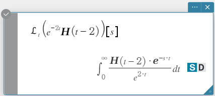
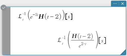
“laplace” is the command for the Laplace transform, and “invLaplace” is the command for the inverse of Laplace transform.
Syntax: laplace \(\mathcal{L}_t (f(t))[s]\)
　　\(f(t)\): expression
　　\(t\): Variable with respect to which the expression is transformed
　　\(s\): parameter of the transform
　　　invLaplace \(\mathcal{L}_s^{-1} (L(s))[t]\)
　　\(L(s)\): expression
　　\(s\): Variable with respect to which the expression is transformed
　　\(t\): parameter of the transform

fourier, invFourier

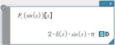
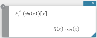
“fourier” is the command for the Fourier transform, and “invFourier” is the command for the inverse Fourier transform.
Syntax: fourier \(~ Ϝ_x (f(x))[w]\)
　　invFourier \(~ Ϝ_w^{-1} (f(w))[x]\)
　　\(x\): Variable with respect to which the expression is transformed
　　\(w\): parameter of the transform

FFT, IFFT

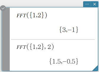
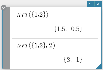
“FFT” is the command for the fast Fourier transform, and “IFFT” is the command for the inverse fast Fourier transform.
The \(2^n\) data value is required to run FFT and IFT. FFT and IFFT are calculated numerically.
Syntax: FFT(list) or FFT(list, m)
　　IFFT(list) or IFFT(list, m)

• Data size must be \(2^n\) for n = 1, 2, 3, …
• The value for m is optional. It can be from 0 to 2, indicating the FFT parameter to use: 0 (Signal Processing), 1 (Pure Math), 2 (Data Analysis).